Bulk salt solution
The very basics of GROMACS through a simple example
The objective of this tutorial is to use the open-source code GROMACS to perform a simple molecular dynamics simulation. The system is a bulk solution of water mixed with sodium (Na+) and sulfate (SO42-) ions.
This tutorial illustrates several major ingredients of molecular dynamics simulations, such as energy minimization, thermostating, NVT and NPT equilibration, and trajectory visualization.
Struggling with your molecular simulations project?
Get guidance for your GROMACS simulations. Contact us for personalized advice for your project.
This tutorial is compatible with the 2024.2 GROMACS version.
The input files
In order to run the present simulation using GROMACS, we need the 3 following files (or sets of files):
A configuration file (.gro) containing the initial positions of the atoms and the box dimensions.
A topology file (.top) specifying the location of the force field files (.itp).
An input file (.mdp) containing the parameters of the simulation (e.g. temperature, timestep).
The specificity of the present tutorial is that both configuration and topology files were prepared with homemade Python scripts, see Write topology using Python. In principle, it is also possible to prepare the system using GROMACS functionalities, such as gmx pdb2gmx, gmx trjconv, or gmx solvate. This will be done in the next tutorial, Protein in electrolyte.
1) The configuration file (.gro)
For the present simulation, the initial atom positions and box size are given in a conf.gro file (Gromos87 format) that you can download by clicking here. Save the conf.gro file in a folder.
The conf.gro file looks like this:
 Na2SO4 solution
 2846
    1  SO4   O1    1   2.608   3.089   2.389
    1  SO4   O2    2   2.562   3.181   2.150
    1  SO4   O3    3   2.388   3.217   2.339
    1  SO4   O4    4   2.425   2.980   2.241
    1  SO4   S1    5   2.496   3.117   2.280
 (...)
  719  Sol  OW1 2843   3.220   2.380   1.540
  719  Sol  HW1 2844   3.279   2.456   1.540
  719  Sol  HW2 2845   3.279   2.304   1.540
  719  Sol  MW1 2846   3.230   2.380   1.540
3.36000   3.36000   3.36000
The first line Na2SO4 solution is just a comment, the second line is the total number of atoms, and the last line is the box dimension in nanometer, here 3.36 nm by 3.36 nm by 3.36 nm. Between the second and the last lines, there is one line per atom. Each line indicates, from left to right:
the residue ID, with all the atoms from the same SO42- ion sharing the same residue ID,
the residue name,
the atom name,
the atom ID,
the atom position: x, y, and z coordinates in nanometer.
Note that the format of a .gro file is fixed, and each column is in a fixed position.
The conf.gro file can be visualized using VMD by typing in the terminal:
vmd conf.gro
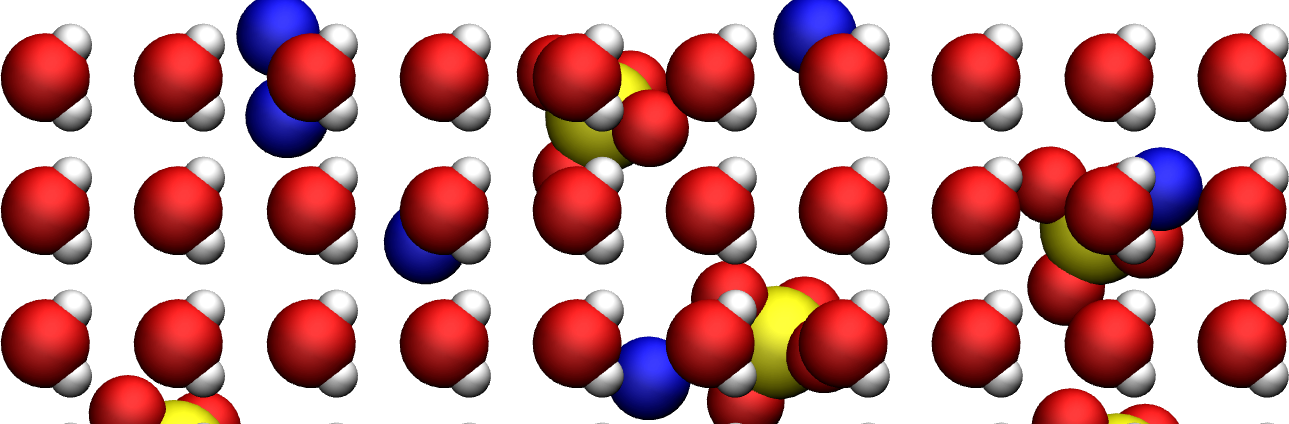
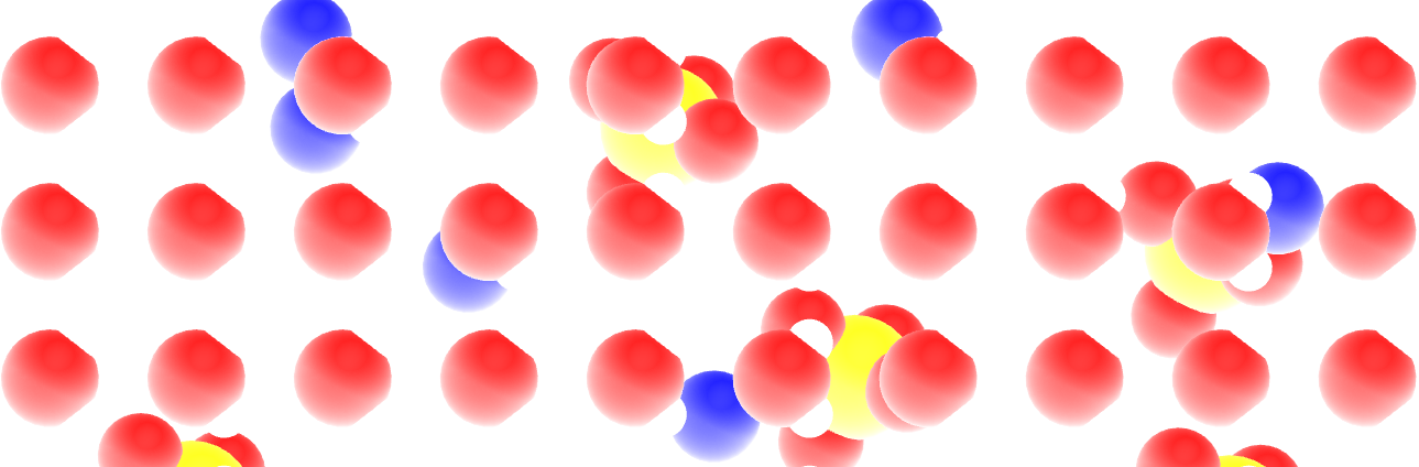
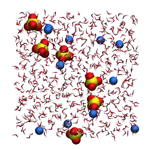
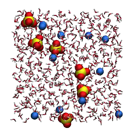
Figure: SO42- ions, Na+ ions, and water molecules. Oxygen atoms are in red, hydrogen in white, sodium in blue, and sulfur in yellow. For better rendering, the atom representation and colors were modified with respect to the default VMD representation. If you want to obtain the same rendering, you can follow this VMD tutorial from the LAMMPS tutorials webpage to obtain a similar rendering.
As can be seen using VMD, the water molecules are arranged in a quite unrealistic and regular manner, with all dipoles facing in the same direction, and possibly wrong distances between some of the molecules and ions. This will be fixed during energy minimization.
2) The topology files (.top .itp)
The topology file contains information about the interactions of the different atoms and molecules. You can download it by clicking here. Place it in the same folder as the conf.gro file. The topol.top file looks like that:
#include "ff/forcefield.itp"
#include "ff/h2o.itp"
#include "ff/na.itp"
#include "ff/so4.itp"

[ System ]
Na2SO4 solution

[ Molecules ]
SO4 6
Na 12
SOL 701
The 4 first lines are used to include the values of the parameters that are given in 4 separate files located in the ff/ folder (see below).
The rest of the topol.top file contains the system name (Na2SO4 solution), and the list of the residues. Here there is 6 SO42- ions, 12 Na+ ions, and 701 water molecules. It is crucial that the order and number of residues in the topology file match the order of the conf.gro file. If you open the conf.gro file, you can see that indeed the first 30 lines beyond to the 6 SO42- residues, the next 12 lines to the 12 Na+ residues, and that the remaining lines concern the water molecules.
Create a folder named ff/ next to the conf.gro and the topol.top files, and copy forcefield.itp, h2o.itp, na.itp, and so4.itp in it. These four files contain information about the atoms (names, masses, changes, Lennard-Jones coefficients) and residues (bond and angular constraints) for all the species that are involved here.
For instance, the forcefield.itp file contains a line that specifies the combination rules as comb-rule 2, which corresponds to the well-known Lorentz-Berthelot rule, where \(\epsilon_{ij} = \sqrt{\epsilon_{ii} \epsilon_{jj}}\) and \(\sigma_{ij} = (\sigma_{ii}+\sigma_{jj})/2\) [9, 10]:
[ defaults ]
; nbfunc  comb-rule  gen-pairs  fudgeLJ  fudgeQQ
1       2          no         1.0      0.833
The fudge parameters specify how the pair interaction between fourth neighbors in a residue are handled, which is not relevant for the small residues considered here. The forcefield.itp file also contains the list of atoms, and their respective charge in the units of the elementary charge \(e\), as well as their respective Lennard-Jones parameters \(\sigma\) (in nanometer) and \(\epsilon\) (in kJ/mol):
[ atomtypes ]
; name  at.num  mass      charge  ptype  sigma    epsilon
Na    11      22.9900   1.0000  A      0.23100  0.45000
OS     8      15.9994  -1.0000  A      0.38600  0.12
SO    16      32.0600   2.0000  A      0.35500  1.0465
HW     1       1.0079   0.5270  A      0.00000  0.00000
OW     8      15.9994   0.0000  A      0.31650  0.77323
MW     0       0.0000  -1.0540  D      0.00000  0.00000
Here the ptype is used to differential the real atoms (A), such as hydrogens and oxygens, from the virtual and massless site of the four-point water model (D).
Finally, the h2o.itp, na.itp, and so4.itp files contain information about the residues, such as their exact compositions, which pairs of atoms are connected by bonds as well as the parameters for these bonds. In the case of the SO42-, for instance, the sulfur atom forms a bond of equilibrium distance \(0.152~\text{nm}\) and rigidity constant \(3.7656 \mathrm{e}4 ~ \text{kJ/mol/nm}^2\) with each of the four oxygen atoms:
[ bonds ]
;  ai   aj  funct   c0         c1
    1    5    1   0.1520   3.7656e4
    2    5    1   0.1520   3.7656e4
    3    5    1   0.1520   3.7656e4
    4    5    1   0.1520   3.7656e4
3) The input file (.mdp)
The input file contains instructions about the simulation, such as
In this tutorial, 4 different input files will be written to perform respectively an energy minimization of the salt solution, an equilibration in the NVT ensemble (i.e. with fixed box size), an equilibration in the NPT ensemble (i.e. with changing box size), and finally a production run.
Input files will be placed in an inputs/ folder that must be created next to ff/.
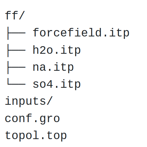
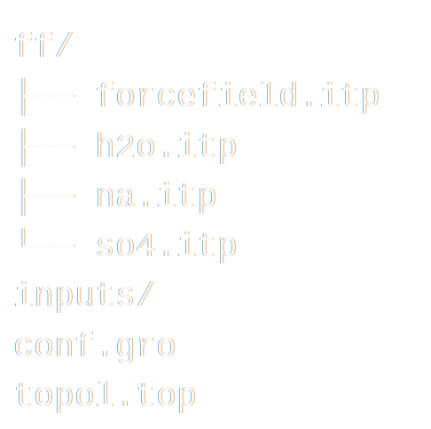
Figure: Structure of the folder with the .itp, .gro, and .top files.
The rest of the tutorial focuses on writing the input files and performing the molecular dynamics simulation.
Energy minimization
It is clear from the configuration (.gro) file that the molecules and ions are currently in a quite unphysical configuration. It would be risky to directly start the molecular dynamics simulation as atoms would undergo huge forces and accelerate, and the system could eventually explode.
To bring the system into a more favorable state, let us perform an energy minimization which consists in moving the atoms until the forces between them are reasonable.
Open a blank file, call it min.mdp, and save it in the inputs/ folder. Copy the following lines into min.mdp:
integrator = steep
nsteps = 5000
These two commands specify to GROMACS that the algorithm to be used is the steepest-descent which moves the atoms following the direction of the largest forces until one of the stopping criteria is reached [13]. The nsteps command specifies the maximum number of steps to perform.
To visualize the trajectory of the atoms during the minimization, let us also add the following command to the input file:
nstxout = 10
The nstxout parameter requests GROMACS to print the atom positions every 10 steps in a .trr trajectory file that can be read by VMD. We now have a very minimalist input script, let us try it. From the terminal, type:
gmx grompp -f inputs/min.mdp -c conf.gro -p topol.top -o min -pp min -po min
gmx mdrun -v -deffnm min
The grompp command is used to preprocess the files in order to prepare the simulation. The grompp command also checks the validity of the files. By using the -f, -c, and -p keywords, we specify which input, configuration, and topology files must be used, respectively. The other keywords -o, -pp, and -po are used to specify the names of the output that will be produced during the run.
The mdrun command calls the engine performing the computation from the preprocessed files (which is recognized thanks to the -deffnm keyword). The -v option enables verbose for more information printed in the terminal.
If everything works, you should see something like:
:-) GROMACS - gmx mdrun, 2023.2 (-:
Executable:   /usr/bin/gmx
Data prefix:  /usr
(...)
Steepest Descents converged to machine precision in 961 steps,
but did not reach the requested Fmax < 10.
Potential Energy  = -4.4659062e+04
Maximum force     =  2.2164763e+02 on atom 15
Norm of force     =  4.5976703e+01
The information printed in the terminal indicates us that energy minimization has been performed, even though the precision that was asked from the default parameters were not reached. We can ignore this message, as long as the final energy is large and negative, the simulation will work just fine.
The final potential energy is large and negative, and the maximum force is as small as \(220 ~ \text{kJ/mol/nm}\) (about 0.4 pN). Everything seems alright. Let us visualize the trajectories of the atoms during the minimization step using VMD by typing in the terminal:
vmd conf.gro min.trr
Figure: Movie showing the motion of the atoms during the energy minimization.
Note for VMD users
You can avoid having molecules cut in half by the periodic boundary conditions by rewriting the trajectory using:
gmx trjconv -f min.trr -s min.tpr -o min_whole.trr -pbc whole
Then, select the group of your choice for the output.
One can see that the molecules reorient themselves into more energetically favorable positions, and that the distances between the atoms are being progressively homogenized.
Let us have a look at the evolution of the potential energy of the system. To do so, we can use the gmx energy command of GROMACS. In the terminal, type:
gmx energy -f min.edr -o potential-energy-minimization.xvg
Choose potential (in my case I have to type 5), then press Enter twice.
Here, the portable energy file min.edr produced by GROMACS during the minimization run is used, and the result is saved in the potential-energy-minimization.xvg file.
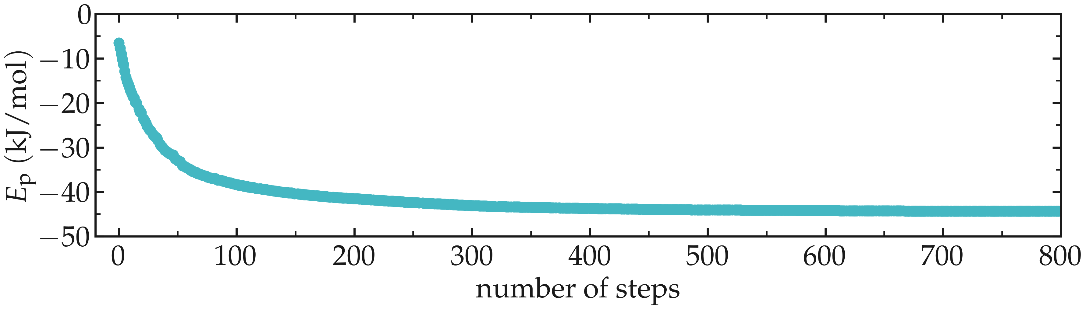
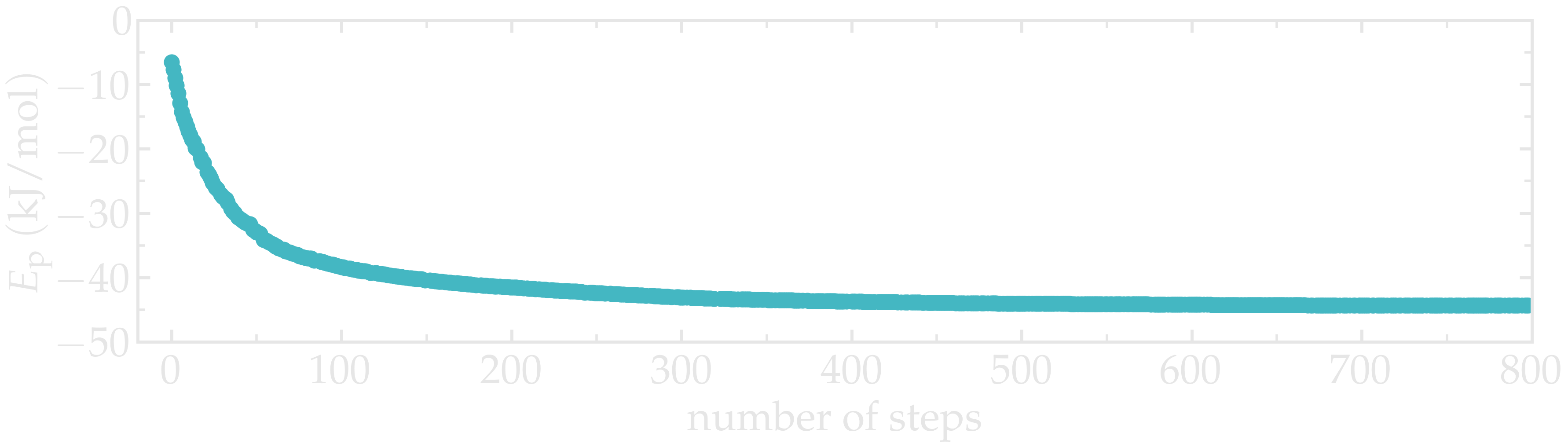
Figure: Evolution of the potential energy \(E_\text{p}\) as a function of the number of steps during energy minimization.
One can see from the energy plot that the potential energy is initially huge and positive, which is the consequence of atoms being too close from one another, as well as molecules being wrongly oriented. As the minimization progresses, the potential energy rapidly decreases and reaches a large and negative value, which is usually the sign that the atoms are located at appropriate distances from each other.
Thank to the energy minimization, the system is now in a favorable state and the molecular dynamics simulation can be started safely.
Minimalist NVT input file
Let us first perform a short (20 picoseconds) equilibration in the NVT ensemble. In the NVT ensemble, the number of atoms (N) and the volume (V) are maintained fixed, and the temperature of the system (T) is adjusted using a thermostat.
Let us write a new input script called nvt.mdp, and save it in the inputs/ folder. Copy the following lines into it:
integrator = md
nsteps = 20000
dt = 0.001
Here, the molecular dynamics (md) integrator is used, this is a leap-frog algorithm integrating Newton equations of motion. A number of 20000 steps with a timestep dt equal of \(0.001 ~ \text{ps}\) will be performed.
Let us also ask GROMACS to print the trajectory in a compressed xtc file every 1000 steps, or every 1 ps, by adding the following line to nvt.mdp:
nstxout-compressed = 1000
Let us also control the temperature throughout the simulation using the v-rescale thermostat, which is the Berendsen thermostat with an additional stochastic term [14].
tcoupl = v-rescale
ref-t = 360
tc-grps = system
tau-t = 0.5
The v-rescale thermostat is known to give a proper canonical ensemble. Here, we also specified that the thermostat is applied to the entire system using the tc-grps option and that the damping constant for the thermostat, tau-t, is equal to 0.5 ps.
Note that the relatively high temperature of 360 K has been chosen here to reduce the viscosity of the solution and decrease the equilibration duration.
We now have a minimalist input file for performing the first NVT simulation. Run it by typing in the terminal:
gmx grompp -f inputs/nvt.mdp -c min.gro -p topol.top -o nvt -pp nvt -po nvt
gmx mdrun -v -deffnm nvt
Here -c min.gro ensures that the previously minimized configuration is used as a starting point.
After the completion of the simulation, we can ensure that the system temperature indeed reached the value of 360 K by using the energy command of GROMACS. In the terminal, type:
gmx energy -f nvt.edr -o temperature-nvt-minimal.xvg
and choose temperature.
From the generated temperature-nvt-minimal.xvg file, one can see that temperature started from 0 K, which was expected since the atoms have no velocity during a minimization step, and reaches a temperature slightly larger than the requested 360 K after a duration of a few picoseconds.
In general, it is better to perform a longer equilibration, but simulation durations are kept as short as possible for these tutorials.
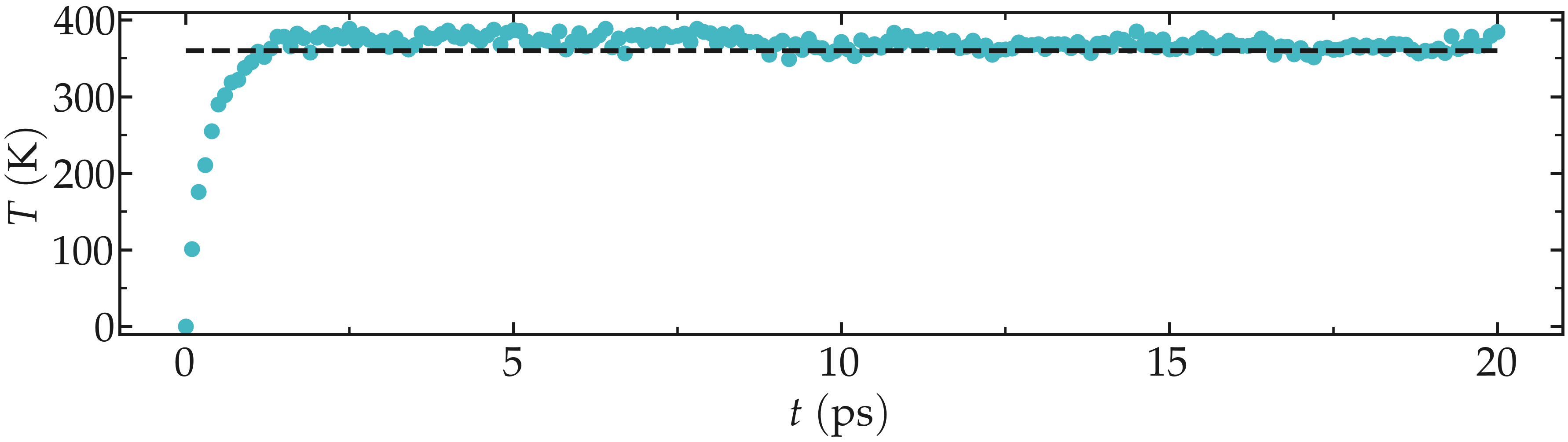
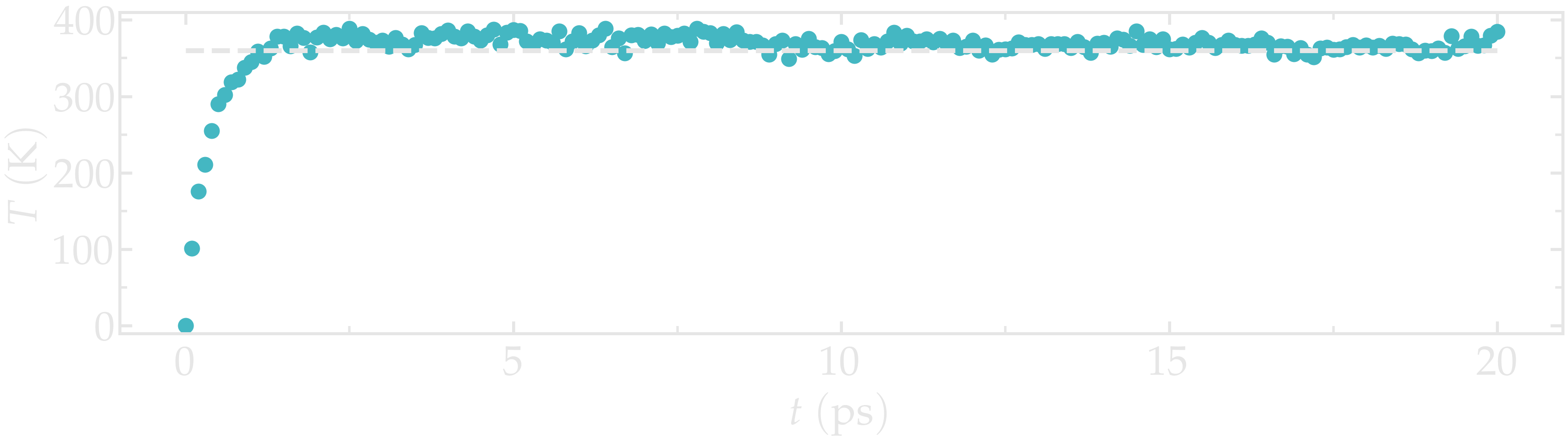
Figure: Evolution of the temperature \(T\) as a function of the time \(t\) during the NVT equilibration. The dashed line is the requested temperature of 360 K.
Improving the NVT input
So far, very few commands have been placed in the .mdp input file, meaning that most of the instructions have been taken by GROMACS from the default parameters. You can find what parameters were used during the last nvt run by opening the new nvt.mdp file that has been created in the main folder. Exploring this new nvt.mdp file shows us that, for instance, plain cut-off Coulomb interactions have been used:
(...)
; Method for doing electrostatics
coulombtype = Cut-off
(...)
For this system, computing the long-range Coulomb interactions is necessary, because electrostatic forces between charged particles decay slowly, as the inverse of the square of the distance between them, \(1/r^2\).
In addition, the thermostating of the system should be improved, given that the temperature of the system is slightly larger than the desired temperature. For instance, separate thermostats can be applied to the water molecules and the ions.
Let us improve the input used for the NVT step. First, in the nvt.mdp file, let us impose the calculation of long-range electrostatic, by the use of the long-range fast smooth particle-mesh ewald (SPME) electrostatics with Fourier spacing of \(0.1~\text{nm}\), order of 4, and cut-off of \(1~\text{nm}\) [15, 16]:
coulombtype = pme
fourierspacing = 0.1
pme-order = 4
rcoulomb = 1.0
Here, the cut-off rcoulomb separates the short-range interactions from the long-range interactions. Long-range interactions are treated in the reciprocal space, while short-range interactions are computed directly.
Let us also impose how the short-range van der Waals interactions should be treated by GROMACS, as well as the cut-off rvdw of \(1~\text{nm}\):
vdw-type = Cut-off
rvdw = 1.0
Let us use the LINCS algorithm to constrain the hydrogen bonds [17]. The water molecules will thus be treated as rigid, which is generally better given the fast vibration of the hydrogen bonds.
constraint-algorithm = lincs
constraints = hbonds
continuation = no
Let us also use separate temperature baths for the water molecules and the ions. Here, the ions are included in the default GROMACS group called non-water. Within nvt.mdp, replace the following lines:
tcoupl = v-rescale
ref-t = 360
tc-grps = system
tau-t = 0.5
by:
tcoupl = v-rescale
tc-grps = Water non-Water
tau-t = 0.5 0.5
ref-t = 360 360
Now, the same temperature \(T = 360 ~ \text{K}\) is imposed to the two groups with the same characteristic time \(\tau = 0.5 ~ \text{ps}\).
Let us also specify the neighbor searching parameters:
cutoff-scheme = Verlet
nstlist = 10
ns_type = grid
Let us give an initial kick to the atom so that the initial total velocities give the desired temperature of 360 K instead of 0 K as previously:
gen-vel = yes
gen-temp = 360
Finally, let us cancel the translational of the center of mass of the system:
comm_mode = linear
comm_grps = system
Run again GROMACS using this new input script. One difference with the previous (minimalist) NVT run is the temperature at the beginning of the run. The final temperature is also much closer to the desired temperature of 360 K.
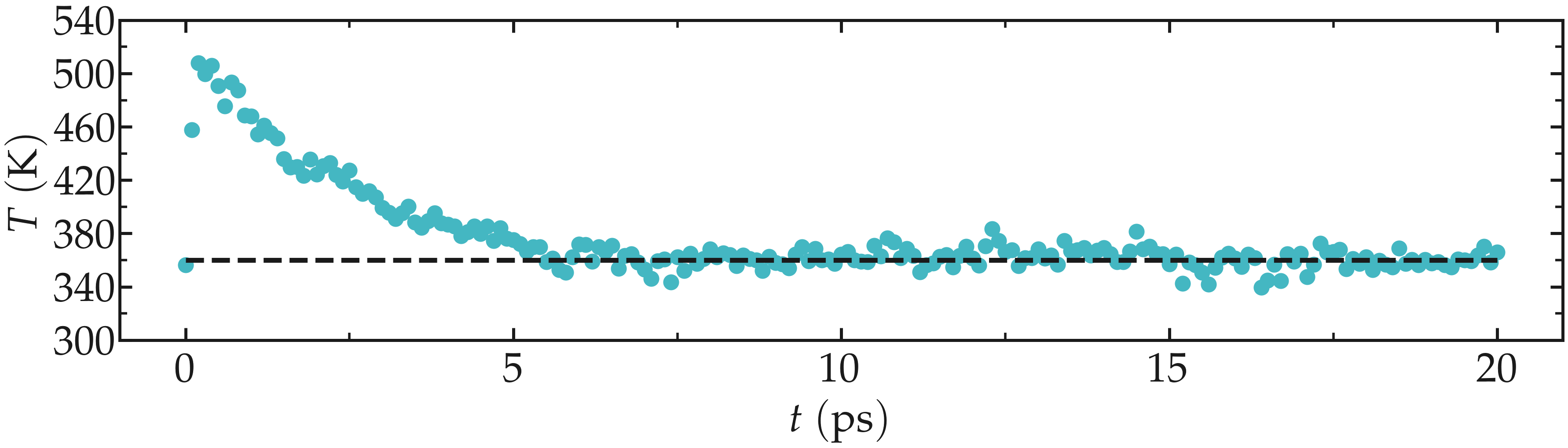
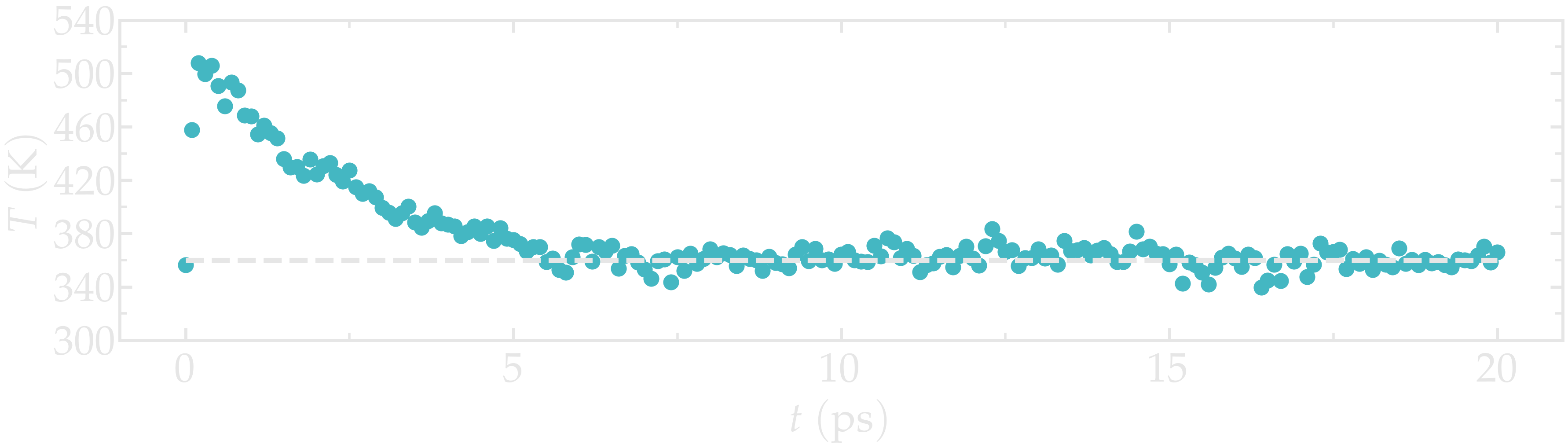
Figure: Evolution of the temperature as a function of the time during the NVT equilibration.
Adjust the density using NPT
Now that the temperature of the system is properly equilibrated, let us continue the simulation using the NPT ensemble, where the pressure of the system is imposed by a barostat and the volume of the box is allowed to relax. During NPT relaxation, the density of the fluid should converge toward its equilibrium value. Create a new input script, call it npt.mdp, and copy the following lines in it:
integrator = md
nsteps = 80000
dt = 0.001

comm_mode = linear
comm_grps = system

cutoff-scheme = Verlet
nstlist = 10
ns_type = grid

nstlog = 100
nstenergy = 100
nstxout-compressed = 1000

vdw-type = Cut-off
rvdw = 1.0

coulombtype = pme
fourierspacing = 0.1
pme-order = 4
rcoulomb = 1.0

constraint-algorithm = lincs
constraints = hbonds

tcoupl = v-rescale
ld-seed = 48456
tc-grps = Water non-Water
tau-t = 0.5 0.5
ref-t = 360 360

pcoupl = C-rescale
Pcoupltype = isotropic
tau_p = 1.0
ref_p = 1.0
compressibility = 4.5e-5
The main difference with the previous NVT script is the addition of the isotropic C-rescale pressure coupling with a target pressure of 1 bar [18]. Another difference is the addition of the nstlog and nstenergy commands to control the frequency at which information is printed in the log file and in the energy file (edr). Note also the removing the gen-vel commands, because the atoms already have a velocity.
Run the NPT equilibration using:
gmx grompp -f inputs/npt.mdp -c nvt.gro -p topol.top -o npt -pp npt -po npt
gmx mdrun -v -deffnm npt
Let us have a look a the temperature, the pressure, and the volume of the box during the NPT step using the gmx energy command 3 consecutive times:
gmx energy -f npt.edr -o temperature-npt.xvg
gmx energy -f npt.edr -o pressure-npt.xvg
gmx energy -f npt.edr -o density-npt.xvg
Choose respectively temperature, pressure and density. This is what I see:
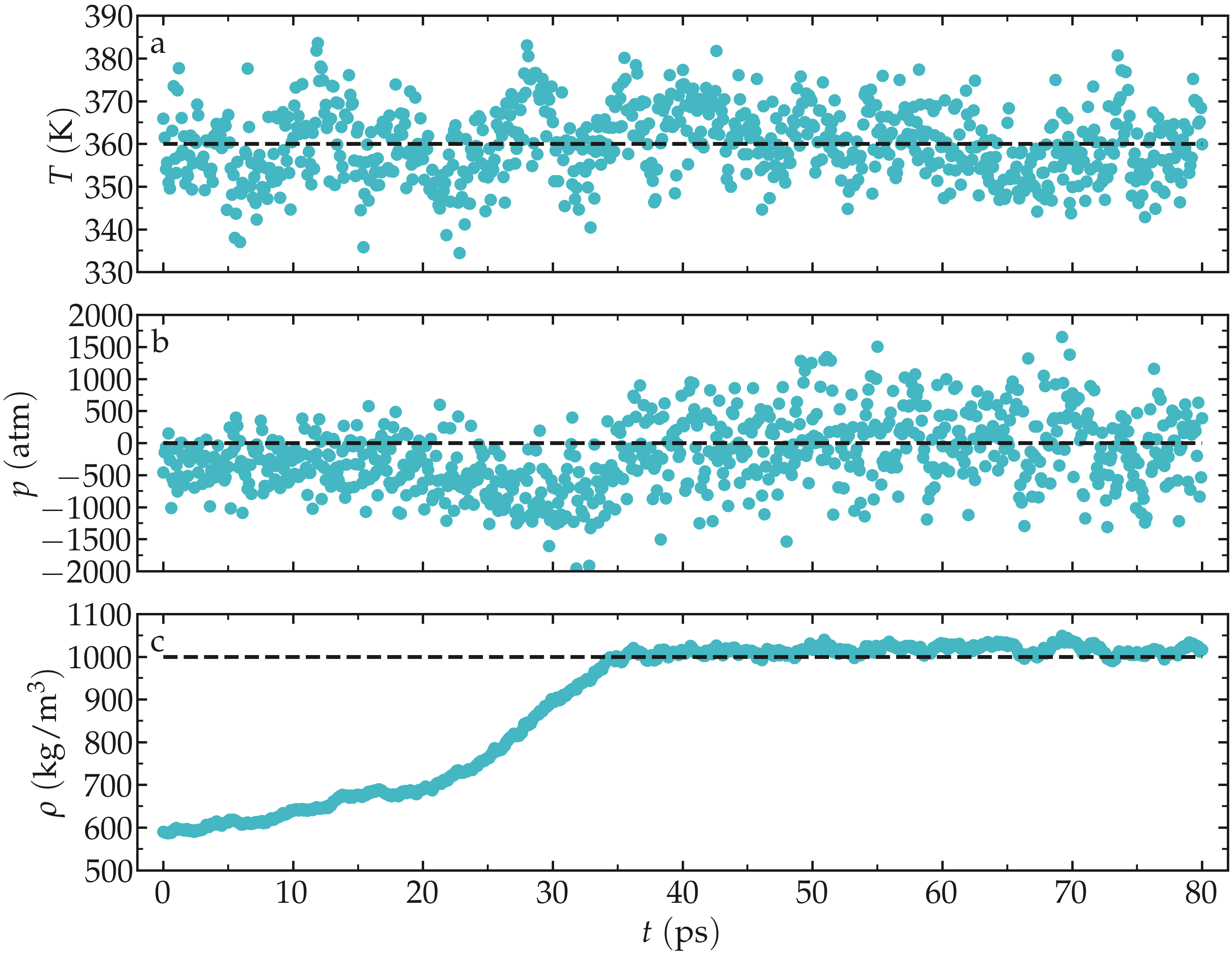
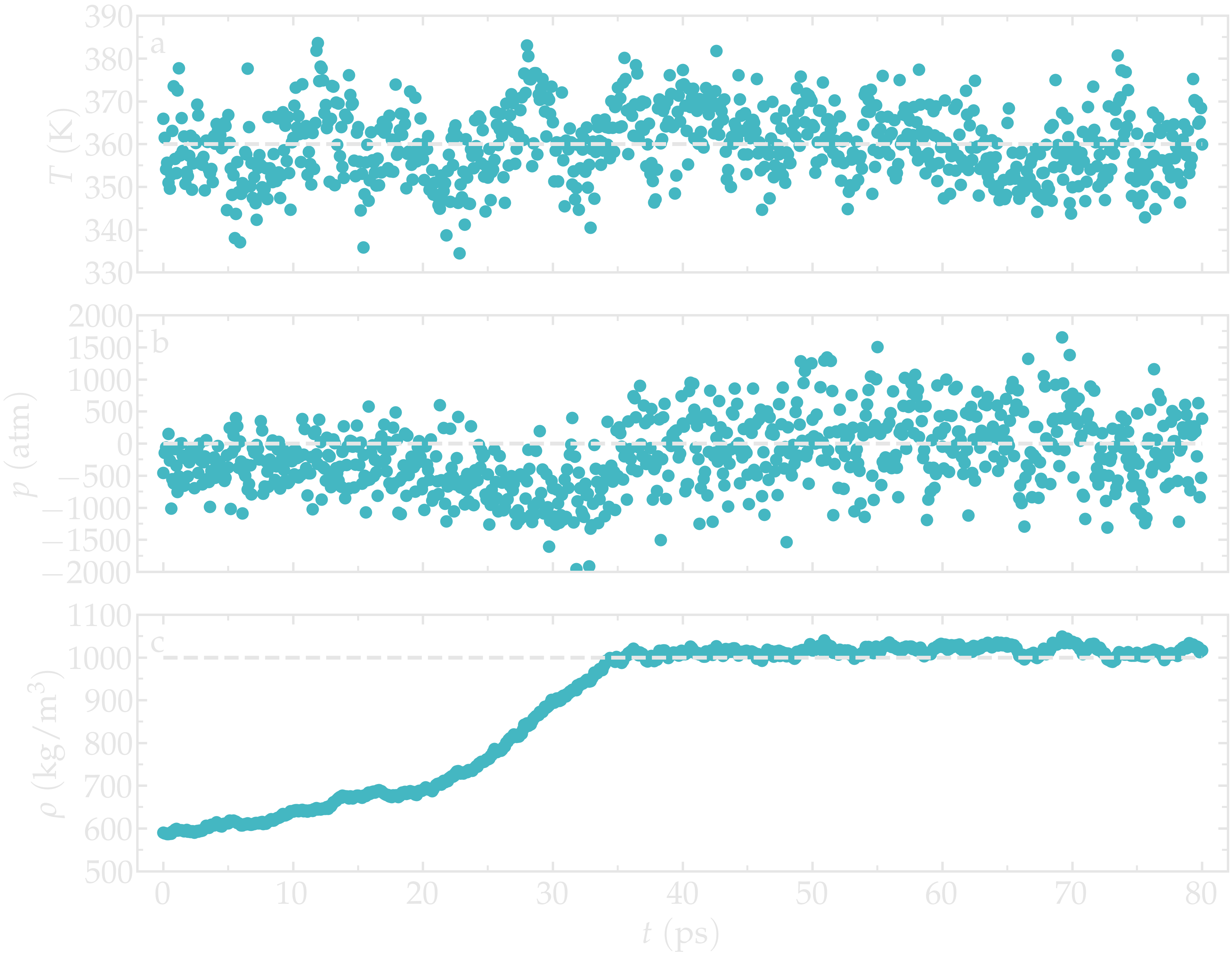
Figure: Evolution of the temperature \(T\) (a), pressure \(p\) (b), and fluid density \(\rho\) (c) as a function of the time during the NPT equilibration.
The results show that the temperature remains well controlled during the NPT run, and that the fluid density was initially too small, i.e. \(\rho \approx 600\,\mathrm{kg}/\mathrm{m}^3\). Due to the change in volume induced by the barostat, the fluid density gently reaches its equilibrium value of about \(1000\,\mathrm{kg}/\mathrm{m}^3\) after approximately 40 pico-seconds. Once the system has reached its equilibrium density, the pressure stabilizes itself near the desired value of 1 bar.
The pressure curve reveals large oscillations in the pressure, with the pressure alternating between large negative values and large positive values. These large oscillations are typical in molecular dynamics, and not a source of concern here.
Radial distribution function
Let us perform a \(400~\text{ps}\) run in the NVT ensemble, during which the atom positions will be printed every pico-second. The trajectory will then be used to measure radial distribution functions and probe the solvation environment of the ions.
Create a new input file within the inputs/ folder, call it production.mdp, and copy the following lines into it:
integrator = md
nsteps = 400000
dt = 0.001

comm_mode = linear
comm_grps = system

cutoff-scheme = Verlet
nstlist = 10
ns_type = grid

nstlog = 100
nstenergy = 100
nstxout-compressed = 1000

vdw-type = Cut-off
rvdw = 1.0

coulombtype = pme
fourierspacing = 0.1
pme-order = 4
rcoulomb = 1.0

constraint-algorithm = lincs
constraints = hbonds

tcoupl = v-rescale
ld-seed = 48456
tc-grps = Water non-Water
tau-t = 0.5 0.5
ref_t = 360 360
Run it using:
gmx grompp -f inputs/production.mdp -c npt.gro -p topol.top -o production -pp production -po production
gmx mdrun -v -deffnm production
When the simulation is completed, let us compute the radial distribution functions between \(\text{Na}^+\) and \(\text{H}_2\text{O}\), \(\text{SO}_4^{2-}\) and \(\text{H}_2\text{O}\), as well as in between \(\text{H}_2\text{O}\) molecules. This can be done using the gmx rdf command as follows:
gmx rdf -f production.xtc -s production.tpr -o na-sol-rdf.xvg
Selecting the sodium ions, and then the water. Repeat the same operation for the sulfate and water, and for the water and water. For the water-water RDF, it is better to exclude the intra-molecular contribution using the -excl option, as follows:
gmx rdf -f production.xtc -s production.tpr -o sol-sol-rdf.xvg -excl
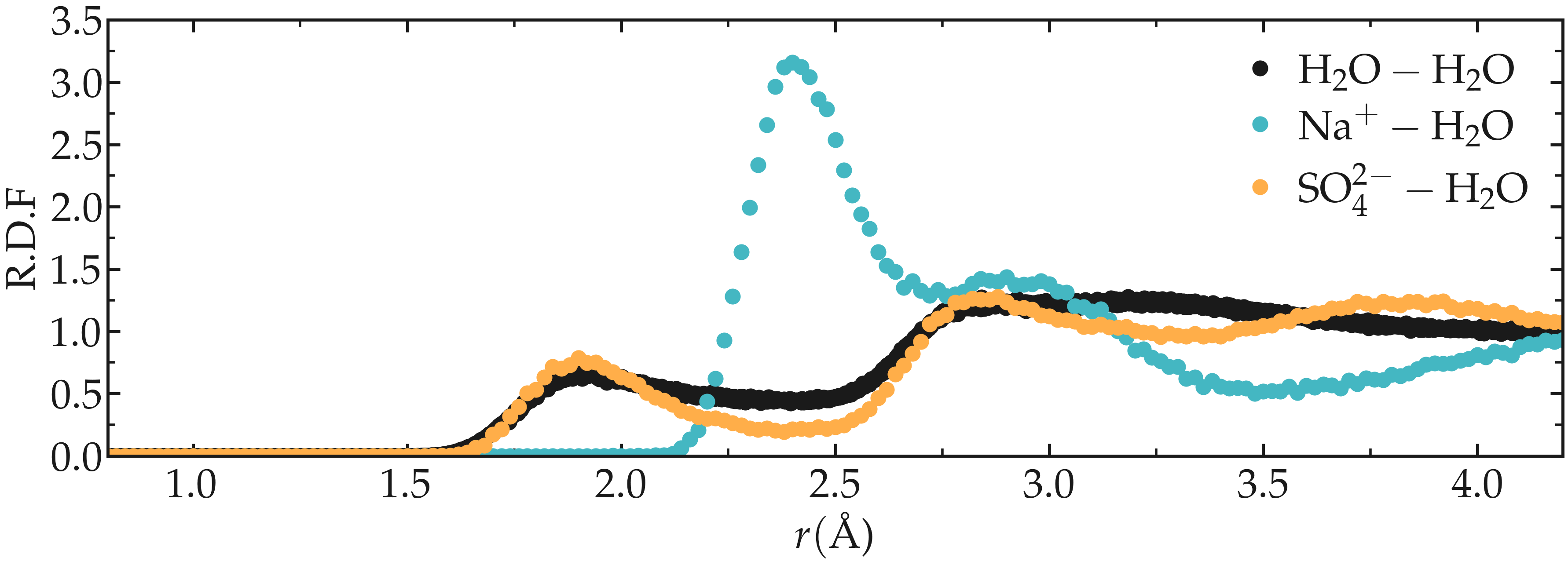
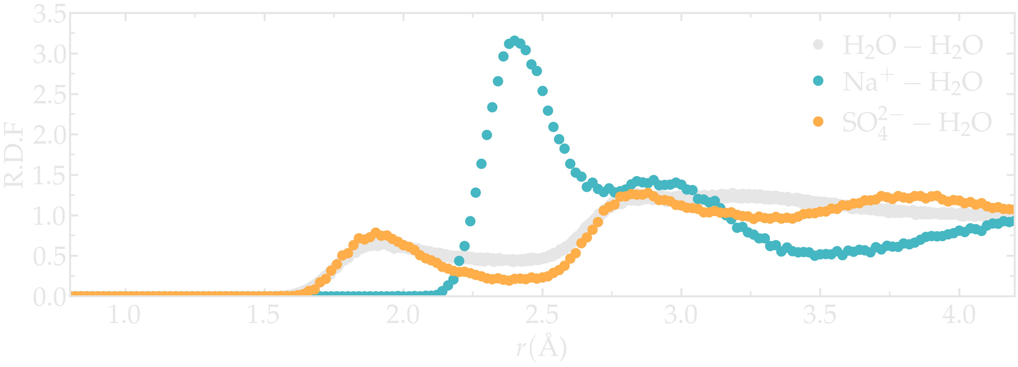
Figure: Radial distribution functions (RDF) as calculated between sodium and water, between sulfate and water, and finally between water and water.
The radial distribution functions highlight the typical distance between the different species of the fluid. For instance, it can be seen that there is a strong hydration layer of water around sodium ions at a typical distance of \(2.4 ~ \text{Å}\) from the center of the sodium ion.
Mean square displacement
To probe the system dynamics, let us compute the mean square displacement for all 3 species. For the sulfate ion, type:
gmx msd -f production.xtc -s production.tpr -o so4-msd.xvg
Select the \(\text{SO}_4^{2-}\) ions (in my case, it is done by typing 2), and then press ctrl D. Repeat the same operation for the sodium ions and for the water molecules.
The slope of the MSD in the limit of long times gives an estimate of the diffusion coefficient, following \(D = \text{MSD} / 2 d t\), where \(d = 3\) is the dimension of the system. Here, I find a value of \(1.4 \mathrm{e}-5 ~ \text{cm}^2/\text{s}\) for the diffusion coefficient of the sulfur ions.
Repeat the same for \(\text{Na}^+\) and water.
For sodium, I find a value of \(1.6 \mathrm{e}-5 ~ \text{cm}^2/\text{s}\) for the diffusion coefficient, and for water \(5.3 \mathrm{e}-5 ~ \text{cm}^2/\text{s}\). For comparison, the experimental diffusion coefficient of pure water at temperature \(T = 360~\text{K}\) is \(7.3 \mathrm{e}-5 ~ \text{cm}^2/\text{s}\) [19]. In the presence of ions, the diffusion coefficient of water is expected to be reduced.
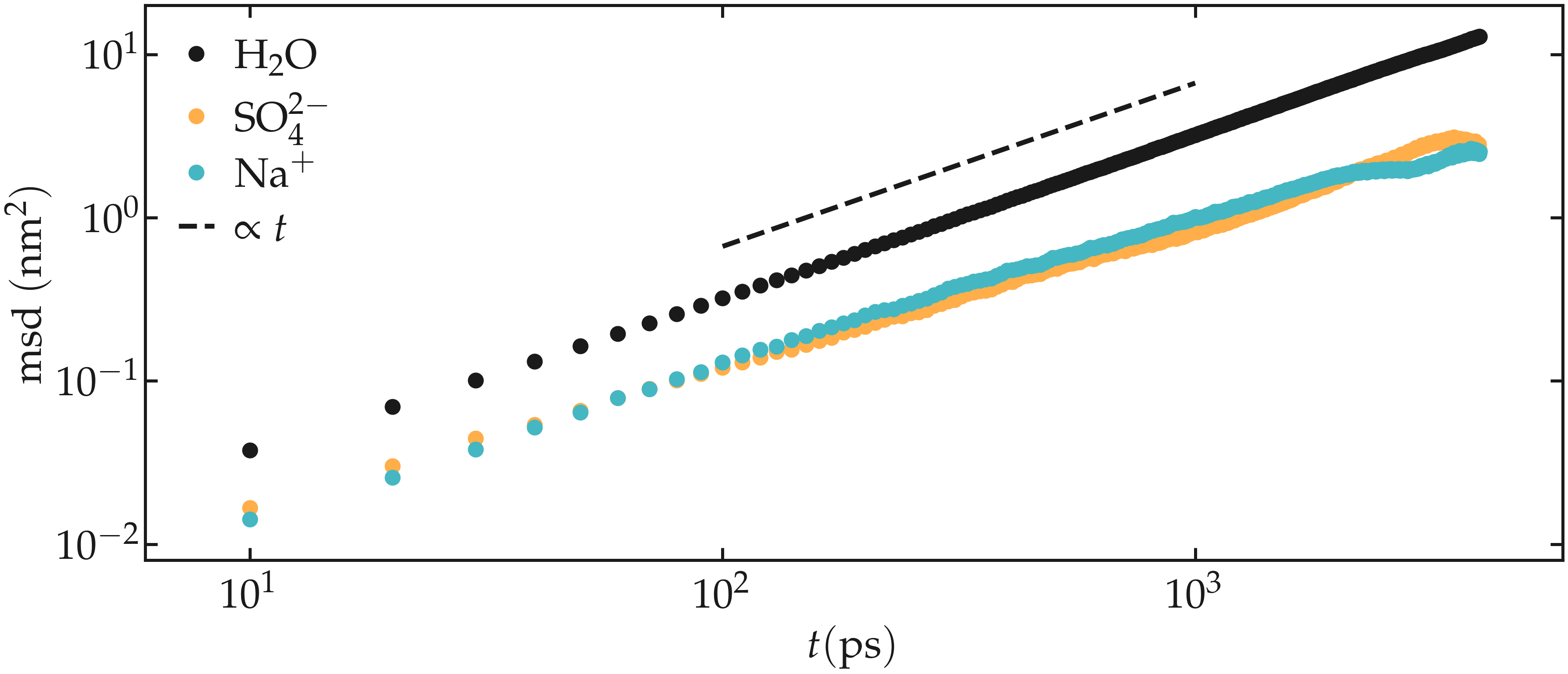
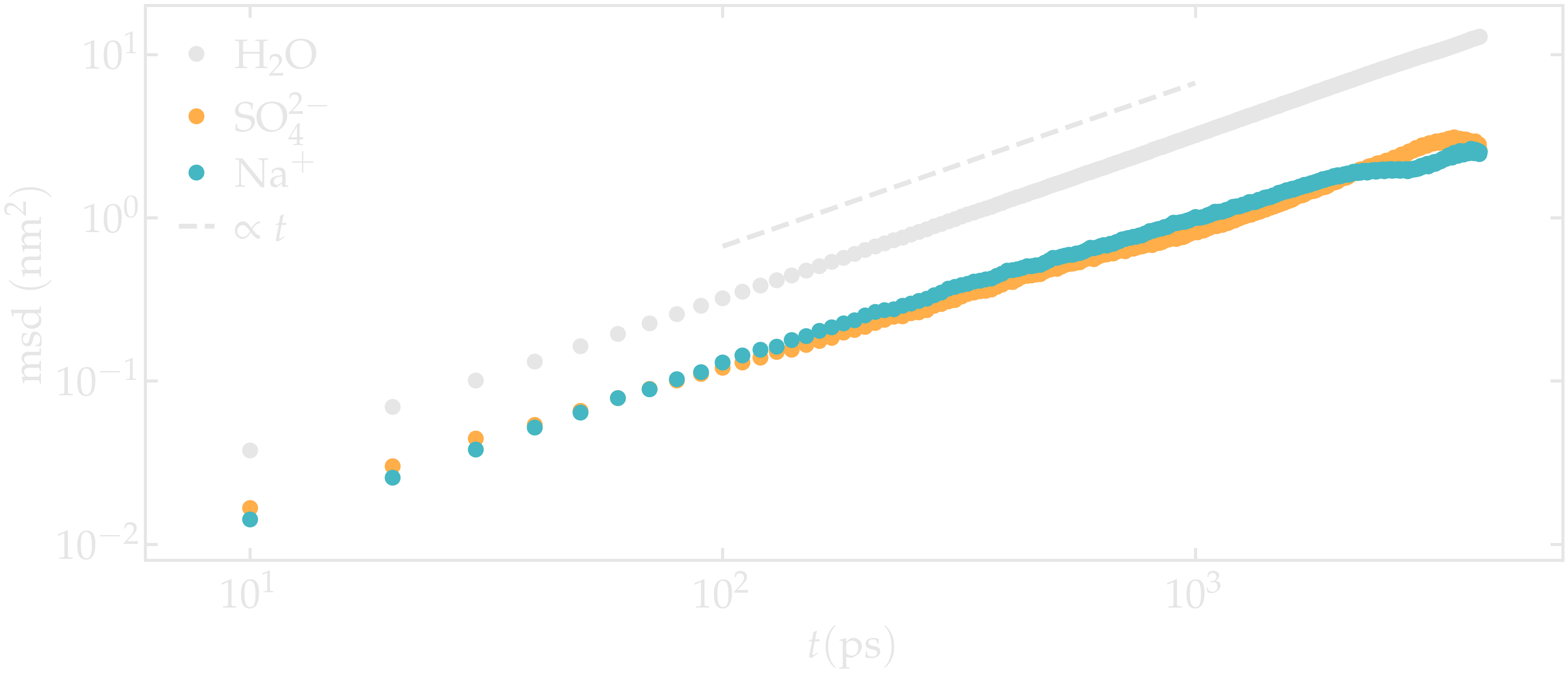
Figure: Mean square displacement (msd) for the three species. The dashed line highlight the proportionality between msd and time \(t\) which is expected at long times, when the system reaches the diffusive regime.
About diffusion coefficient measurement in molecular simulations
In principle, diffusion coefficients obtained from the MSD in a finite-sized box must be corrected, but this is beyond the scope of the present tutorial [20].
You can access all the input scripts and data files that are used in these tutorials from GitHub.