Solvation energy

Calculating the free energy of solvation of a graphene-like molecule

The objective of this tutorial is to use GROMACS to perform a molecular simulation of a large molecule in water. By progressively switching off the interactions between the molecule and water, the free energy of solvation will be calculated.

The large and flat molecule used here is a graphene-like and discoid molecule named hexabenzocoronene (HBC) of formula \(\text{C}_{42}\text{H}_{18}\). The TIP4P/epsilon model is used for the water [27].

If you are completely new to GROMACS, I recommend that you follow this tutorial on a simple Bulk salt solution first.

Struggling with your molecular simulations project?

Get guidance for your GROMACS simulations. Contact us for personalized advice for your project.

This tutorial is compatible with the 2024.2 GROMACS version.

Input files

Create two folders side-by side. Name the two folders preparation/ and solvation/, and go to preparation/.

Download the configuration files for the HBC molecule by clicking this page, and save it in the preparation/ folder. The molecule was downloaded from the atb on the automated topology builder (ATB) [28].

Create the configuration file

First, let us convert the .pdb file into a .gro file within a cubic box of lateral size 3 nanometers using the gmx trjconv command. Type the following command in a terminal:

gmx trjconv -f FJEW_allatom_optimised_geometry.pdb -s FJEW_allatom_optimised_geometry.pdb -o hbc.gro -box 3 3 3 -center

Select system for both centering and output.

Figure: HBC molecule as seen with VMD with carbon atoms in gray and hydrogen atoms in white. The honeycomb structure of the HBC is similar to that of graphene.

Alternatively, you can download the hbc.gro I have generated, and continue with the tutorial.

Create the topology file

Create a folder named ff/ within the preparation/ folder. Copy the force field parameters from the following zip file by clicking here. Both FJEW_GROMACS_G54A7FF_allatom.itp file and gromos54a7_atb.ff/ folder were downloaded from the atb.

Then, let us write the topology (top) file by simply creating a blank file named topol.top within the preparation/ folder. Copy the following lines into topol.top:

#include "ff/gromos54a7_atb.ff/forcefield.itp"
#include "ff/FJEW_GROMACS_G54A7FF_allatom.itp"

[ system ]
Single HBC molecule

[ molecules ]
FJEW 1

Solvate the HBC in water

Let us add water molecules to the system. First, download the tip4p water configuration (.gro) file here, and copy it in the preparation/ folder. This is a fourth point water model with additional massless site where the charge of the oxygen atom is placed. Then, in order to add tip4p water molecules to both .gro and .top file, use the gmx solvate command as follows:

gmx solvate -cs tip4p.gro -cp hbc.gro -o solvated.gro -p topol.top

The new solvated.gro file contains all 8804 atoms from the HBC molecule (called FJEW) and the water molecules. A new line SOL 887 also appeared in the topology .top file:

[ molecules ]
FJEW 1
SOL 887

Alternatively, you can download the solvated.gro file I have generated by clicking here, and continue with the tutorial.

Finally, save the topology file for the water, the h2o.itp file, in the ff/ folder and add the #include “ff/h2o.itp” line to the topol.top file:

#include "ff/gromos54a7_atb.ff/forcefield.itp"
#include "ff/FJEW_GROMACS_G54A7FF_allatom.itp"
#include "ff/h2o.itp"

System equilibration

The system is now ready for the simulations. Let us first equilibrate it before measuring the solvation energy of the HBC molecule.

Energy minimization

Create an inputs/ folder inside the preparation/ folder, and create a new blank file called min.mdp in it. Copy the following lines into min.mdp:

integrator = steep
nsteps = 50

nstxout = 10

cutoff-scheme = Verlet
nstlist = 10
ns_type = grid

couple-intramol=yes

vdw-type = Cut-off
rvdw = 1.2

coulombtype = pme
fourierspacing = 0.1
pme-order = 4
rcoulomb = 1.2

constraint-algorithm = lincs
constraints = hbonds

All these lines have been seen in the previous tutorials. In short, with this input script, GROMACS will perform a steepest descent by updating the atom positions according to the largest forces directions, until the energy and maximum force reach a reasonable value.

Apply the minimization to the solvated box using gmx grompp and gmx mdrun:

gmx grompp -f inputs/min.mdp -c solvated.gro -p topol.top -o min -pp min -po min -maxwarn 1
gmx mdrun -v -deffnm min

Here, the -maxwarn 1 option is used to ignore a WARNING from GROMACS about some issue with the force field. For this tutorial, we can safely ignore this WARNING.

Let us visualize the atom trajectories during the minimization step using VMD by typing:

vmd solvate.gro min.trr

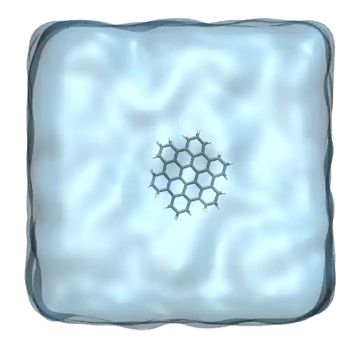
Figure: The system after energy minimization showing the HBC molecule in water. The water is represented as a transparent field.

NVT and NPT equilibration

Let us perform successively a NVT and a NPT relaxation steps. Copy the nvt.mdp and the npt.mdp files into the inputs folder, and run them both using:

gmx grompp -f inputs/nvt.mdp -c min.gro -p topol.top -o nvt -pp nvt -po nvt -maxwarn 1
gmx mdrun -v -deffnm nvt
gmx grompp -f inputs/npt.mdp -c nvt.gro -p topol.top -o npt -pp npt -po npt -maxwarn 1
gmx mdrun -v -deffnm npt

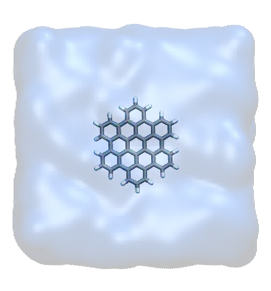
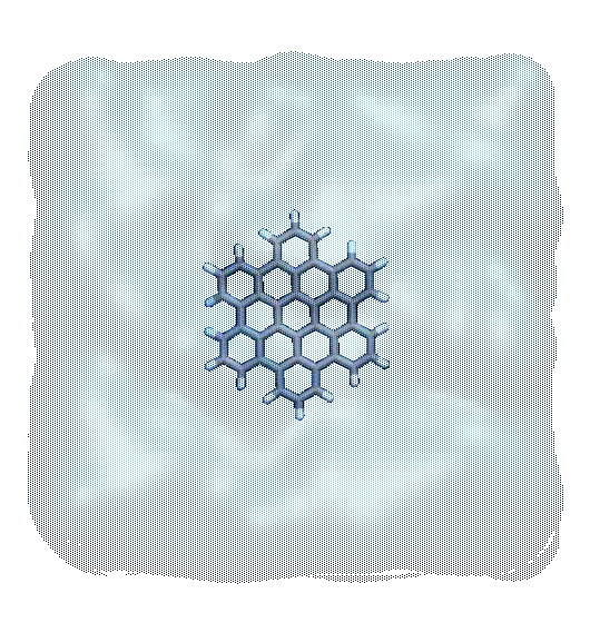
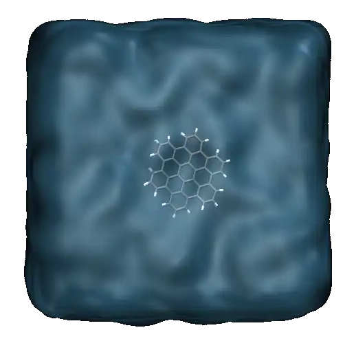
Figure: Movie showing the motion of the atoms during the NVT and NPT equilibration steps. For clarity, the water molecules are represented as a continuum field.

Solvation energy measurement

Files preparation

The equilibration of the system is complete. Let us perform the solvation free energy calculation, for which 21 independent simulations will be performed.

About free energy calculation

The interactions between the HBC molecule and the water are progressively turned-off, thus effectively mimicking the HBC molecule moving from bulk water to vacuum. Then, the free energy difference between the fully solvated and the fully decoupled configurations is measured.

Within the solvation/ folder, create an inputs/ folders, and copy the following input file into it: equilibration.mdp.

This input file starts similarly as the inputs previously used in this tutorial, with the exception of the integrator. Instead of the md integrator, a sd for stochastic dynamics integrator:

integrator = sd
nsteps = 20000
dt = 0.001

This stochastic integrator creates a Langevin dynamics by adding a friction and a noise term to Newton equations of motion. The sd integrator also serves as a thermostat, therefore tcoupl is set to No:

tcoupl = No
ld-seed = 48456
tc-grps = Water non-Water
tau-t = 0.5 0.5
ref-t = 300 300

A stochastic integrator can be a better option for free energy measurements, as it generates a better sampling, while also imposing a strong control of the temperature. This is particularly useful when the molecules are completely decoupled.

The rest of the input deals with the progressive decoupling of the HBC molecule from the water:

free_energy = yes
vdw-lambdas = 0.0 0.1 0.2 0.3 0.4 0.5 0.6 0.7 0.8 0.9 1.0 1.0 1.0 1.0 1.0 1.0 1.0 1.0 1.0 1.0 1.0
coul-lambdas = 0.0 0.0 0.0 0.0 0.0 0.0 0.0 0.0 0.0 0.0 0.0 0.1 0.2 0.3 0.4 0.5 0.6 0.7 0.8 0.9 1.0

The vdw-lambdas is used to turn-off (when vdw-lambdas = 0) or turn-on (when vdw-lambdas = 1) the van der Waals interactions, and the coul-lambdas is used to turn-off/turn-on the Coulomb interactions.

Here, there are 21 possible states, from vdw-lambdas = coul-lambdas = 0.0, where the HBC molecule is fully decoupled from the water, to vdw-lambdas = coul-lambdas = 1.0, where the HBC molecule is fully coupled to the water. All the other state correspond to situation where the HBC molecule is partially coupled with the water.

The sc-alpha and sc-power options are used to turn-on a soft core repulsion between the HBC and the water molecules. This is necessary to avoid overlap between the decoupled atoms.

The init-lambda-state is an integer that specifies which values of vdw-lambdas and coul-lambdas is used. When init-lambda-state, then vdw-lambdas = coul-lambdas = 0.0. 21 one independent simulations will be performed, each with a different value of init-lambda-state:

init-lambda-state =  0

The couple-lambda0 and couple-lambda1 are used to specify that indeed interaction are turn-off when the lambdas are 0, and turn-on when the lambdas as 1:

couple-lambda0 = none
couple-lambda1 = vdw-q

The parameter nstdhdl controls the frequency at which information are being printed in a .xvg file during the production run.

nstdhdl = 0

For the equilibration, there is no need of printing information. For the production runs, a value \(>0\) will be used for nstdhdl.

The 2 last lines impose that lambda points will be written out, and which molecule will be used for calculating solvation free energies:

calc_lambda_neighbors = -1
couple-moltype = FJEW

Let us create a second input file almost identical to equilibration.mdp. Duplicate equilibration.mdp, name the duplicated file production.mdp. Within production.mdp, simply change nstdhdl from 0 to 100, so that information about the state of the system will be printed by GROMACS every 100 step during the production runs.

Finally, copy the previous topol.top file from the preparation/ folder into solvation/ folder. In oder to avoid duplicating the force field folder ff/, modify the path to the .itp files as follow:

#include "../preparation/ff/gromos54a7_atb.ff/forcefield.itp"
#include "../preparation/ff/FJEW_GROMACS_G54A7FF_allatom.itp"
#include "../preparation/ff/h2o.itp"

[ system ]
Single HBC molecule in water

[ molecules ]
FJEW 1
SOL 887

Perform a 21-step loop

We need to a total of 2 x 21 simulations, 2 simulations per value of init-lambda-state. This can be done using a small bash script with the sed (for stream editor) command.

Create a new bash file fine within the ‘solvation/’ folder, call it local-run.sh can copy the following lines in it:

#/bin/bash
set -e

# create folder for analysis
mkdir -p dhdl

# loop on the 21 lambda state
for state in $(seq 0 20)
do
    # create folder for the lambda state
    DIRNAME=lambdastate${state}
    mkdir -p $DIRNAME

    # update the value of init-lambda-state
    newline='init-lambda-state = '$state
    linetoreplace=$(cat inputs/equilibration.mdp | grep init-lambda-state)
    sed -i '/'"$linetoreplace"'/c\'"$newline" inputs/equilibration.mdp
    linetoreplace=$(cat inputs/production.mdp | grep init-lambda-state)
    sed -i '/'"$linetoreplace"'/c\'"$newline" inputs/production.mdp

    gmx grompp -f inputs/equilibration.mdp -c ../preparation/npt.gro -p topol.top -o equilibration -pp equilibration -po equilibration -maxwarn 1
    gmx mdrun -v -deffnm equilibration -nt 4

    gmx grompp -f inputs/production.mdp -c equilibration.gro -p topol.top -o production -pp production -po production -maxwarn 1
    gmx mdrun -v -deffnm production -nt 4

    mv production.* $DIRNAME
    mv equilibration.* $DIRNAME

    # create links for the analysis
    cd dhdl/
        ln -sf ../$DIRNAME/production.xvg md$state.xvg
    cd ..
done

Within this bash script, the variable state increases from 0 to 20 in a for loop. At eash step of the loop, a folder lambdastateX is created, where X goes from 0 to 20. Then, the sed command is used twice to update the value of init-lambda-state in both equilibration.mdp and production.mdp.

Then, GROMACS is used to run the equilibration.mdp script, and then the production.mdp script. When the simulations are done, the generated files are moved into the lambdastateX folder. Finally the ln command creates a link toward the production.xvg file within the dhdl/ folder.

Execute the bash script by typing:

bash createfolders.sh

Completing the 2 x 21 simulations may take a while, depending on your computer. When the simulation is complete, go the dhdl folder, and call the gmx bar command:

gmx bar -f *.xvg

The value of the solvation energy is printed in the terminal. In my case, I see:

DG -64.62 +/- 6.35

This indicate that the solvation energy is of \(-64.6 \pm 6.3~\text{kJ/mol}\). Note however that the present simulations are too short to give a reliable result. To accurately measure the solvation energy of a molecule, you should use much longer equilibration, typically one nanosecond, as well as much longer production runs, typically several nanoseconds.

You can access all the input scripts and data files that are used in these tutorials from GitHub.