Write topology using Python
Use Python to write topology files compatible with GROMACS
The objective of this extra tutorial is to use Python and write simple topology files that are compatible with GROMACS. The system consists in molecules and ions randomly placed in an empty box, and is used as a starting point in bulk-solution-label.
Creating the GRO file
If you are only interested in learning GROMACS, jump directly to the actual GROMACS tutorial bulk-solution-label.
Struggling with your molecular simulations project?
Get guidance for your GROMACS simulations. contact-label for personalized advice for your project.
What is a GRO file?
A .gro file contains the initial positions and names of all the atoms of a simulation. The .gro file also contains the initial box size, and it can be read by GROMACS.
The typical structure of a .gro file is the following:
Name of the system
number-of-atoms
residue-number residue-name atom-name atom-number atom-positions (x3) # first atom
residue-number residue-name atom-name atom-number atom-positions (x3) # second atom
residue-number residue-name atom-name atom-number atom-positions (x3) # third atom
(...)
residue-number residue-name atom-name atom-number atom-positions (x3) # penultimate atom
residue-number residue-name atom-name atom-number atom-positions (x3) # last atom
box-size (x3)
One particularity of .gro file format is that each column must be located at a fixed position, see the GROMACS manual.
Residue definition
About residue
In GROMACS, a residue refers to a group of one or more atoms that are covalently linked and considered as a single unit within a molecule, ion, etc.
Open a blank Python script, call it molecules.py, and copy the following lines in it:
import numpy as np

# define SO4 ion
def SO4_ion():
    Position = np.array([[0.1238,  0.0587,   0.1119], \
        [0.0778,   0.1501,  -0.1263], \
        [-0.0962,   0.1866,   0.0623], \
        [-0.0592,  -0.0506,  -0.0358],\
        [0.0115,   0.0862,   0.0030]])
    Type = ['OS', 'OS', 'OS', 'OS', 'SO']
    Name = ['O1', 'O2', 'O3', 'O4', 'S1']
    Resname = 'SO4'
    return Position, Type, Resname, Name

# define Na ion
def Na_ion():
    Position = np.array([[0, 0, 0]])
    Type = ['Na']
    Name = ['Na1']
    Resname = 'Na'
    return Position, Type, Resname, Name

# define water molecule
def H20_molecule():
    Position = np.array([[ 0.    ,  0.    ,  0.    ], \
        [ 0.05858,  0.0757 ,  0.    ], \
        [ 0.05858, -0.0757 ,  0.    ], \
        [ 0.0104 ,  0.    ,  0.    ]])
    Type = ['OW', 'HW', 'HW', 'MW']
    Name = ['OW1', 'HW1', 'HW2', 'MW1']
    Resname = 'Sol'
    return Position, Type, Resname, Name
Each function corresponds to a residue, and contains the positions, types, and names of all the atoms, as well as the names of the residues. These functions will be called every time we need to place a residue in our system.
The water molecule contains a massless point (TIP4P model) in addition to the oxygen and hydrogens atoms [29].
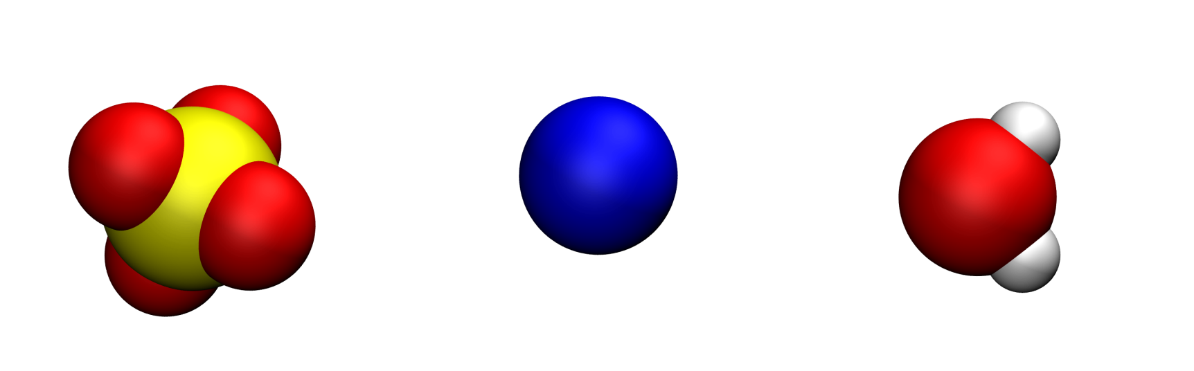
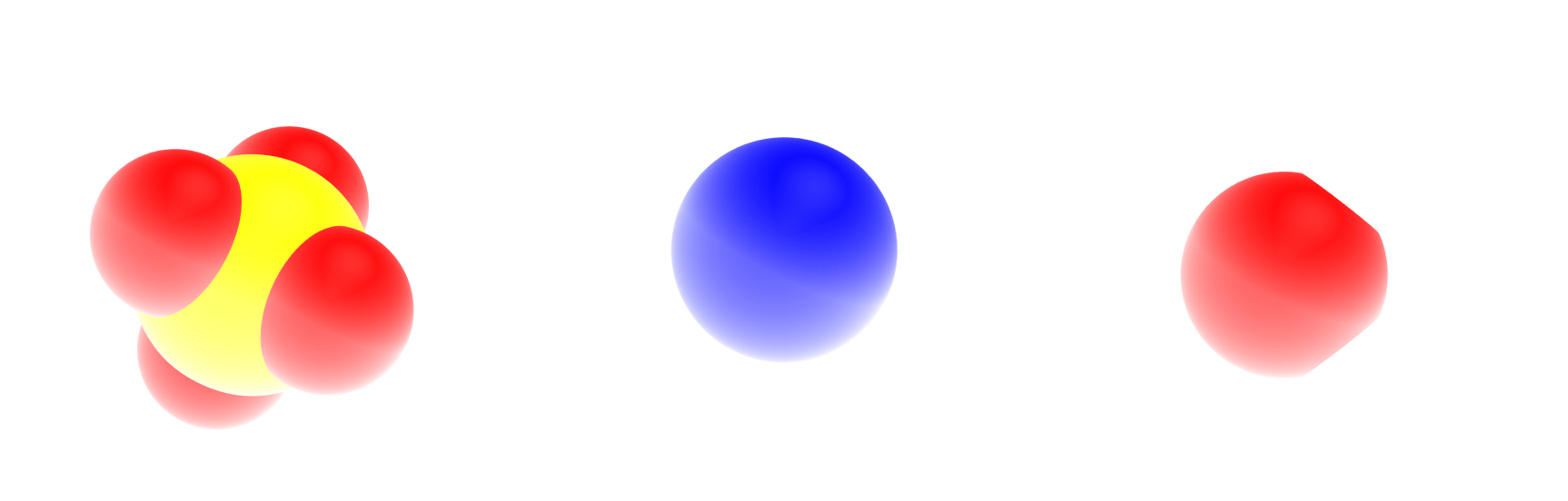
From left to right, the sulfide ion (\(\text{SO}_4^{2-}\)), the sodium ion (\(\text{Na}^{+}\)), and the water molecules (\(\text{H}_2\text{O}\)). Oxygen atoms are in red, hydrogen atoms in white, sodium atoms in blue, and sulfur atoms in yellow. The fourth massless point (MW) of the water molecule is not visible.
Creating the GRO file
Here, we define some of the basic parameters of the simulation, such as the number of residues and the box size.
Next to the molecule.py file, create a new Python file called generategro.py, and copy the following lines into it:
import numpy as np
from molecules import SO4_ion, Na_ion, H20_molecule

# define the box size
Lx, Ly, Lz = [3.36]*3
box = np.array([Lx, Ly, Lz])
Here, box is an array containing the box size along all 3 coordinates of space, respectively Lx, Ly, and Lz. A cubic box of lateral dimension \(3.6 ~ \text{nm}\) is used.
Let us choose a salt concentration, and calculate the number of ions and water molecules accordingly, while also choosing the total number of residues (here I call residue either a molecule or an ion). Add the following to generategro.py:
Mh2o = 0.018053 # kg/mol - water
ntotal = 720 # total number of molecule
c = 1.5 # desired concentration in mol/L
nion = c*ntotal*Mh2o/(3*(1+Mh2o*c)) # desired number for the SO4 ion
nwater = ntotal - 3*nion # desired number of water
Let us also choose typical cutoff distances (in nanometer) for each species. These cutoffs will be used to ensure that no species are inserted too close to one another, as it would make the simulation crash later:
dSO4 = 0.45
dNa = 0.28
dSol = 0.28
Let us initialize several counters and several lists. The lists will be used for storing all the data about the atoms:
cpt_residue = 0
cpt_atoms = 0
cpt_SO4 = 0
cpt_Na = 0
cpt_Sol = 0
all_positions = []
all_resnum = []
all_resname = []
all_atname = []
all_attype = []
Let us first add a number nion of \(\text{SO}_4^{2-}\) ions at random locations. To avoid overlap, let us only insert ion if no other ions is already located at a distance closer than dSO4:
# add SO4 randomly
atpositions, attypes, resname, atnames = SO4_ion()
while cpt_SO4 < np.int32(nion):
    x_com, y_com, z_com = generate_random_location(box)
    d = search_closest_neighbor(np.array(all_positions), atpositions + np.array([x_com, y_com, z_com]), box)
    if d < dSO4:
        add_residue = False
    else:
        add_residue = True
    if add_residue == True:
        cpt_SO4 += 1
        cpt_residue += 1
        for atposition, attype, atname in zip(atpositions, attypes, atnames):
            cpt_atoms += 1
            x_at, y_at, z_at = atposition
            all_positions.append([x_com+x_at, y_com+y_at, z_com+z_at])
            all_resnum.append(cpt_residue)
            all_resname.append(resname)
            all_atname.append(atname)
            all_attype.append(attype)
Here, two functions are used: generate_random_location and search_closest_neighbor. Let us define those two functions. Create a new Python script, call it utils.py, and copy the following lines in it:
import numpy as np
from numpy.linalg import norm

def generate_random_location(box):
    """Generate a random location within a given box."""
    return np.random.rand(3)*box

def search_closest_neighbor(XYZ_neighbor, XYZ_molecule, box):
    """Search neighbor in a box and return the closest distance.

    If the neighbor list is empty, then the box size is returned.
    Periodic boundary conditions are automatically accounted
    """
    if len(np.array(XYZ_neighbor)) == 0:
        min_distance = np.max(box)
    else:
        min_distance = np.max(box)
        for XYZ_atom in XYZ_molecule:
            dxdydz = np.remainder(XYZ_neighbor - XYZ_atom + box/2., box) - box/2.
            min_distance = np.min([min_distance,np.min(norm(dxdydz,axis=1))])
    return min_distance
The generate_random_location function simply generates 3 random values within the box. The search_closest_neighbor looks for the minimum distance between existing atoms (if any) and the new residue.
Let us do the same for the \(\text{Na}^{+}\) ion :
# Import the functions from the utils file
from utils import generate_random_location, search_closest_neighbor

# add Na randomly
atpositions, attypes, resname, atnames = Na_ion()
while cpt_Na < np.int32(nion*2):
    x_com, y_com, z_com = generate_random_location(box)
    d = search_closest_neighbor(np.array(all_positions), atpositions + np.array([x_com, y_com, z_com]), box)
    if d < dNa:
        add_residue = False
    else:
        add_residue = True
    if add_residue == True:
        cpt_Na += 1
        cpt_residue += 1
        for atposition, attype, atname in zip(atpositions, attypes, atnames):
            cpt_atoms += 1
            x_at, y_at, z_at = atposition
            all_positions.append([x_com+x_at, y_com+y_at, z_com+z_at])
            all_resnum.append(cpt_residue)
            all_resname.append(resname)
            all_atname.append(atname)
            all_attype.append(attype)
Let us also insert water molecules on a 3D regular grid with spacing of dSol (only if no overlap exists):
# add water randomly
atpositions, attypes, resname, atnames = H20_molecule()
for x_com in np.arange(dSol/2, Lx, dSol):
    for y_com in np.arange(dSol/2, Ly, dSol):
        for z_com in np.arange(dSol/2, Lz, dSol):
            d = search_closest_neighbor(np.array(all_positions), atpositions + np.array([x_com, y_com, z_com]), box)
            if d < dSol:
                add_residue = False
            else:
                add_residue = True
            if (add_residue == True) & (cpt_Sol < np.int32(nwater)):
                cpt_Sol += 1
                cpt_residue += 1
                for atposition, attype, atname in zip(atpositions, attypes, atnames):
                    cpt_atoms += 1
                    x_at, y_at, z_at = atposition
                    all_positions.append([x_com+x_at, y_com+y_at, z_com+z_at])
                    all_resnum.append(cpt_residue)
                    all_resname.append(resname)
                    all_atname.append(atname)
                    all_attype.append(attype)
            if cpt_Sol >= np.int32(nwater):
                break
print(cpt_Sol, 'out of', np.int32(nwater), 'water molecules created')
Let us ask Python to print a few information such as the actual concentration:
print('Lx = '+str(Lx)+' nm, Ly = '+str(Ly)+' nm, Lz = '+str(Lz)+' nm')
print(str(cpt_Na)+' Na ions')
print(str(cpt_SO4)+' SO4 ions')
print(str(cpt_Sol)+' Sol mols')
Vwater = cpt_Sol/6.022e23*0.018 # kg or litter
Naddion = (cpt_Na+cpt_SO4)/6.022e23 # mol
cion = Naddion/Vwater
print('The ion concentration is '+str(np.round(cion,2))+' mol per litter')
Finally, let us write the configuration (.gro) file:
# write conf.gro
f = open('conf.gro', 'w')
f.write('Na2SO4 solution\n')
f.write(str(cpt_atoms)+'\n')
cpt = 0
for resnum, resname, atname, position  in zip(all_resnum, all_resname, all_atname, all_positions):
    x, y, z = position
    cpt += 1
    f.write("{: >5}".format(str(resnum))) # residue number (5 positions, integer)
    f.write("{: >5}".format(resname)) # residue name (5 characters)
    f.write("{: >5}".format(atname)) # atom name (5 characters)
    f.write("{: >5}".format(str(cpt))) # atom number (5 positions, integer)
    f.write("{: >8}".format(str("{:.3f}".format(x)))) # position (in nm, x y z in 3 columns, each 8 positions with 3 decimal places)
    f.write("{: >8}".format(str("{:.3f}".format(y)))) # position (in nm, x y z in 3 columns, each 8 positions with 3 decimal places)
    f.write("{: >8}".format(str("{:.3f}".format(z)))) # position (in nm, x y z in 3 columns, each 8 positions with 3 decimal places)
    f.write("\n")
f.write("{: >10}".format(str("{:.5f}".format(Lx)))) # box size
f.write("{: >10}".format(str("{:.5f}".format(Ly)))) # box size
f.write("{: >10}".format(str("{:.5f}".format(Lz)))) # box size
f.write("\n")
f.close()
Final system
Run the generategro.py file using Python. This is what appear in the terminal:
701 out of 701 water molecules created
Lx = 3.36 nm, Ly = 3.36 nm, Lz = 3.36 nm
12 Na ions
6 SO4 ions
701 Sol mols
The ion concentration is 1.43 mol per litter
You can check the final system using VMD by typing in a terminal:
vmd conf.gro
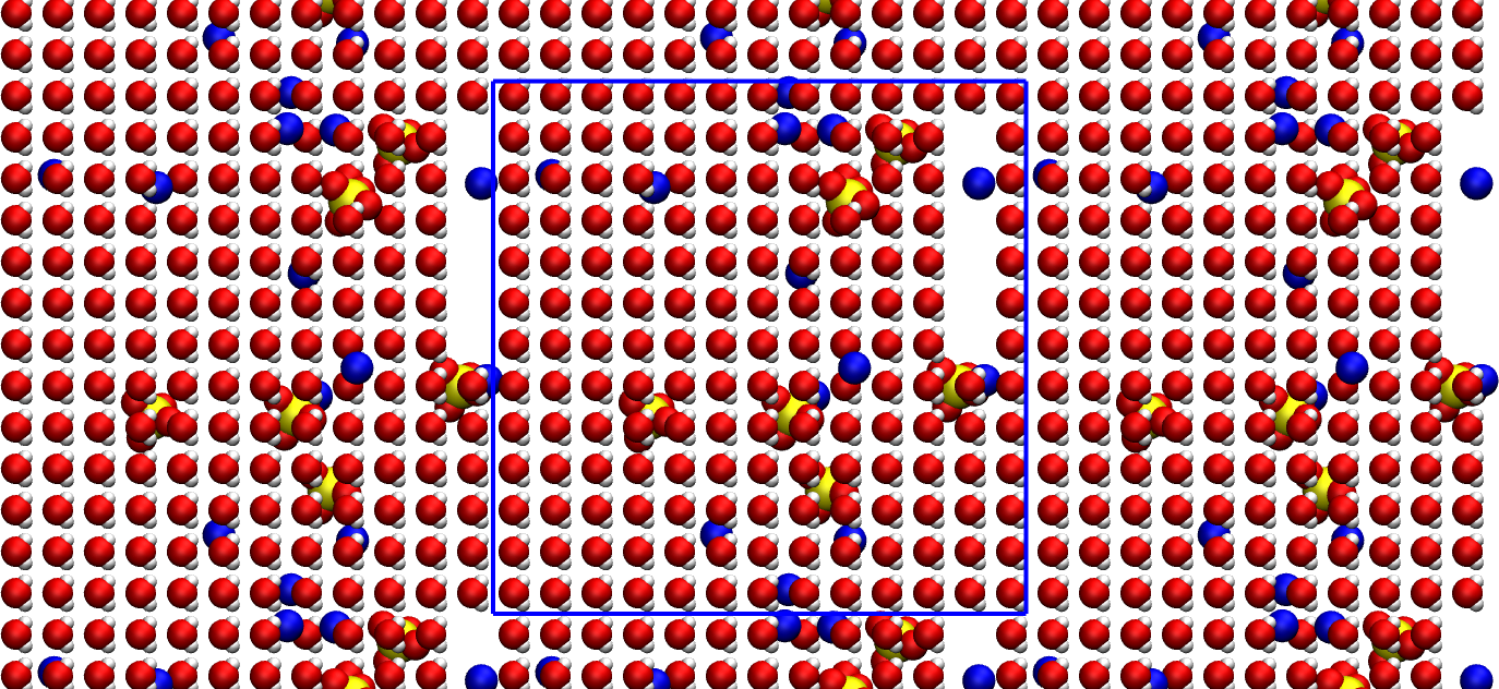
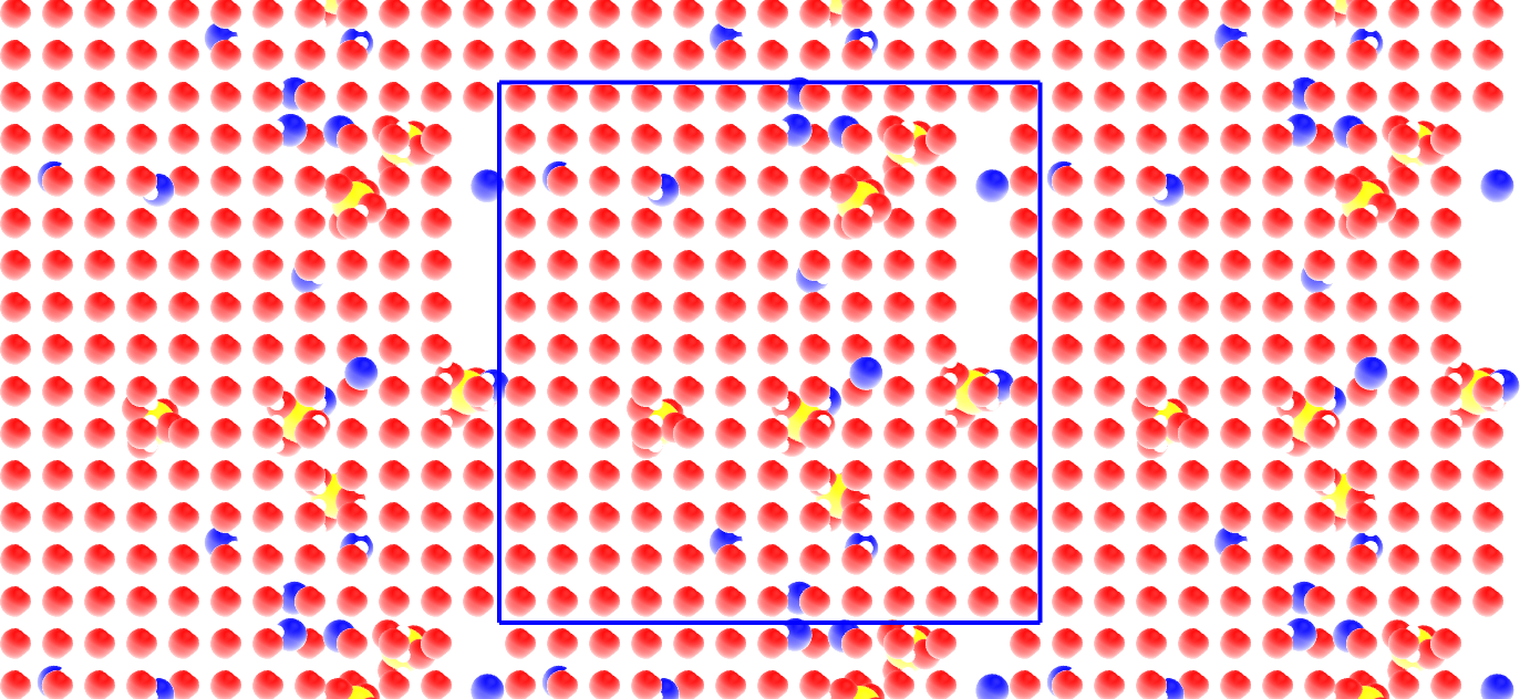
The primary system is located within the blue box. The replicated periodic images are also represented.
There is some vacuum left in the box. It is not an issue as energy minimization and molecular dynamics will help equilibrate the system.
Creating the TOP file
A topology (.top) file defines the parameters required for the simulation, such as masses, Lennard-Jones parameters, or bonds.
Within the same Python script, write:
# write topol.top
f = open('topol.top', 'w')
f.write('#include "ff/forcefield.itp"\n')
f.write('#include "ff/h2o.itp"\n')
f.write('#include "ff/na.itp"\n')
f.write('#include "ff/so4.itp"\n\n')
f.write('[ System ]\n')
f.write('Na2SO4 solution\n\n')
f.write('[ Molecules ]\n')
f.write('SO4 '+ str(cpt_SO4)+'\n')
f.write('Na '+ str(cpt_Na)+'\n')
f.write('SOL '+ str(cpt_Sol)+'\n')
f.close()
Write parameters
Here, the force field parameters (i.e. the .itp files) are written.
Default parameters
Create a folder called ff/. Within ff/, create a new empty file named forcefield.itp, and copy the following in it:
[ defaults ]
; nbfunc  comb-rule  gen-pairs  fudgeLJ  fudgeQQ
  1       2          no         1.0      0.833

[ atomtypes ]
; name  at.num  mass      charge  ptype  sigma    epsilon
  Na    11      22.9900   1.0000  A      0.23100  0.45000
  OS     8      15.9994  -1.0000  A      0.38600  0.12
  SO    16      32.0600   2.0000  A      0.35500  1.0465
  HW     1       1.0079   0.5270  A      0.00000  0.00000
  OW     8      15.9994   0.0000  A      0.31650  0.77323
  MW     0       0.0000  -1.0540  D      0.00000  0.00000

[ bondtypes ]
; i   j   func  b0    kb
  SO  OS  1     0.15  3.7656e4

[ angletypes ]
; i   j   k   func  theta  k0
  OS  SO  OS  1     109.5  520
The forcefield.itp file is used to define basic combination rules, as well as atom types, bond types, and angle types.
With comb-rule = 2, the mixing rule is calculated as \(\epsilon_{ij} = \sqrt{\epsilon_{ii} \epsilon_{jj}}\), \(\sigma_{ij} = (\sigma_{ii}+\sigma_{jj})/2\). FudgeLJ and fudgeQQ are the factors by which to multiply Lennard-Jones and Coulomb 1-4 interactions, respectively. You can refer to the GROMACS manual for more information.
The forcefield.itp file also contains information about the atoms, such their masses and Lennard-Jones parameters sigma and epsilon, as well as some parameters for the bond and angle constraints that will be necessary for the SO4 ions.
Notice that the particle with name MW is of type ‘D’ when all the other particles are of type ‘A’ for atoms. This is because MW is the virtual massless site of our 4 points rigid water model, see this wiki page for details.
Sodium ion
Let us create a file named na.itp for the Sodium ion (na.itp):
[ moleculetype ]
; molname nrexcl
  Na      1

[ atoms ]
; id  at-type  res-nr  res-name  at-name  cg-nr  charge  mass
  1   Na       1       Na        Na1      1      1.000   22.9900
The ‘molecule’ named Na for a residue with one single atom, of type Na and name Na1, charge +1.0 and mass 22.990 g/mol.
Sulfate ion
The file so4.itp for the sulfate ion is more complex than the one for the sodium ion, as the residue is made of 5 atoms that are bonded together and maintained by angular constrained (so4.itp).
The exclusions ensures that atoms from the same residue do not interact through LJ and Coulomb interactions.
[moleculetype]
; name  nrexcl
  SO4   1

[ atoms ]
; id  at-type  res-nr  res-name  at-name  cg-nr  charge  mass
  1   OS       1       SO4       O1       1     -1.000   15.9994
  2   OS       1       SO4       O2       1     -1.000   15.9994
  3   OS       1       SO4       O3       1     -1.000   15.9994
  4   OS       1       SO4       O4       1     -1.000   15.9994
  5   SO       1       SO4       S1       1      2.000   32.0600

[ bonds ]
;  ai   aj  funct   c0         c1
   1    5   1       0.1520     3.7656e4
   2    5   1       0.1520     3.7656e4
   3    5   1       0.1520     3.7656e4
   4    5   1       0.1520     3.7656e4

[ angles ]
;  ai   aj   ak  funct   angle     fc
   1    5    2    1    109.5  520
   1    5    3    1    109.5  520
   1    5    4    1    109.5  520
   2    5    3    1    109.5  520
   2    5    4    1    109.5  520
   3    5    4    1    109.5  520

[exclusions]
1       2       3       4       5
2       1       3       4       5
3       1       2       4       5
4       1       2       3       5
5       1       2       3       4
Water molecule
Finally, create a file named h2o.itp for the water molecule (h2o.itp). Settle parameters are added to ensure that the water molecule remains rigid:
[ moleculetype ]
; molname  nrexcl
SOL      2

[ atoms ]
; id  at-type  res-nr  res-name  at-name  cg-nr  charge  mass
  1   OW       1       SOL       OW1      1      0.000    15.9994
  2   HW       1       SOL       HW1      1      0.527     1.0079
  3   HW       1       SOL       HW2      1      0.527     1.0079
  4   MW       1       SOL       MW1      1     -1.054     0.0000

[ settles ]
; i  funct  doh      dhh
  1  1      0.09572  0.15139

[ virtual_sites3 ]
; Vsite from          funct        a               b
  4     1     2     3     1       0.089608       0.089608

[ exclusions ]
1 2 3 4
2 1 3 4
3 1 2 4
4 1 2 3
To continue and use those files for running a molecular dynamics simulation with GROMACS, go to bulk-solution-label.