Free energy profile
Free energy profile calculation using umbrella sampling and WHAM
The objective of this tutorial is to use GROMACS to perform a molecular simulation, and to calculate the free energy of adsorption of ethanol at a liquid-vapor interface.
A liquid-vapor slab made of water and ethanol molecules is first equilibrated under ambient conditions. Then, umbrella sampling is used to probe the free energy profile of a chosen molecule across the liquid-vapor interface.
If you are completely new to GROMACS, I recommend that you follow this tutorial on a simple bulk-solution-label first.
Struggling with your molecular simulations project?
Get guidance for your GROMACS simulations. contact-label for personalized advice for your project.
This tutorial is compatible with the 2024.2 GROMACS version.
Prepare the input files
Create 3 folders side-by-side named respectively preparation/, adsorption/, and singleposition/. Go to preparation/.
Download the configuration files for the ethanol molecule from the ATB repository (click on All-Atom PDB (optimised geometry)), and place the file BIPQ_allatom_optimised_geometry.pdb in the preparation/ folder.
Create the configuration file
First, let us convert the pdb file into a gro file consisting of a single ethanol molecule at the center of a small box using the gmx trjconv command:
gmx trjconv -f BIPQ_allatom_optimised_geometry.pdb -s BIPQ_allatom_optimised_geometry.pdb -box 0.8 0.8 0.8 -o single_ethanol.gro -center
Select system for both centering and output.
Replicate the ethanol molecule
To create a system with several ethanol molecules, let us replicate the single molecule (4x4x4 times) using genconf:
gmx genconf -f single_ethanol.gro -o replicated_ethanol.gro -nbox 4 4 4
If you open the replicated_ethanol.gro file with VMD, you will see the replicated ethanol molecules.
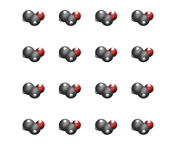
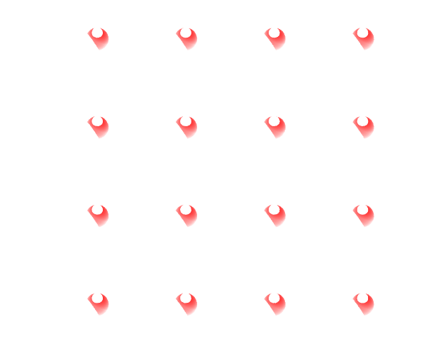
Figure: Replicated ethanol molecules with carbon atoms in gray, oxygen atoms in red, and hydrogen atoms in white.
Create the topology file
Within the preparation/ folder, create a folder named ff/.
From the same page from the ATB repository, download the file named GROMACS G54A7FF All-Atom (ITP file) and place within ff/. Download as well the GROMACS top file named Gromacs 4.5.x-5.x.x 54a7 containing most of the force field parameters. Finally, copy the h2o.itp file for the water molecules in the ff/ folder.
Create a blank file named topol.top within the preparation/ folder, and copy the following lines in it:
#include "ff/gromos54a7_atb.ff/forcefield.itp"
#include "ff/BIPQ_GROMACS_G54A7FF_allatom.itp"
#include "ff/h2o.itp"

[ system ]
Ethanol molecules

[ molecules ]
BIPQ 64
Add the water
Let us add water molecules. First download the tip4p water configuration file here and copy it in the preparation/ folder. Then, in order to add (tip4p) water molecules to both gro and top files, use the gmx solvate command as follows:
gmx solvate -cs tip4p.gro -cp replicated_ethanol.gro -o solvated.gro -p topol.top
In my case, 858 water molecules with residue name SOL were added.
There should be a new line SOL 858 in the topology file topol.top:
[ molecules ]
BIPQ 64
SOL 858
The created solvated.gro file contains the positions of both ethanol and water molecules, it looks like this:
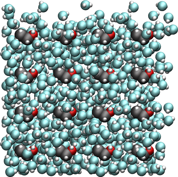
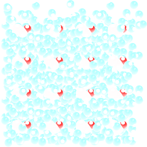
Figure: Replicated ethanol molecules surrounded by water (in light blue color).
To create a liquid-vapor slab, let us increase the box size along the x direction to create a large vacuum area:
gmx trjconv -f solvated.gro -s solvated.gro -box 20.0 3.2 3.2 -o solvated_vacuum.gro -center
Select system for both centering and output.
Alternatively, download the solvated_vacuum.gro file I have generated by clicking here and continue with the tutorial.
Energy minimization
Create a new folder in the preparation/’ folder, call it ‘inputs’, and save the min.mdp and the nvt.mdp files into it.
These 2 files have been seen in the previous tutorials. They contain the GROMACS commands, such as the type of solver to use, the temperature, etc. Apply the minimization to the solvated box using :
gmx grompp -f inputs/min.mdp -c solvated_vacuum.gro -p topol.top -o min -pp min -po min -maxwarn 1
gmx mdrun -v -deffnm min
Here the ‘-maxwarn 1’ allows us to perform the simulation despite GROMACS’ warning about some issue with the force field. Let us visualize the atoms’ trajectories during the minimization step using VMD by typing:
vmd solvated_vacuum.gro min.trr
During energy minimization, the molecules move until the forces between the atoms are reasonable.
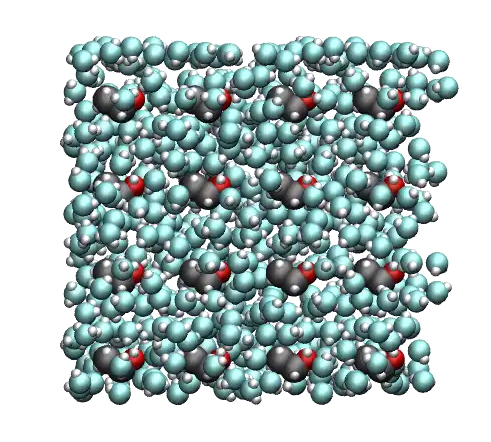
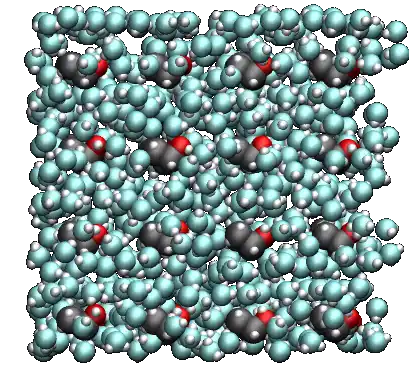
Figure: Movie showing the motion of the atoms during the energy minimization. The two fluid/vacuum interfaces are on the left and or the right sides, respectively.
Note for VMD users
You can avoid having molecules cut in half by the periodic boundary conditions by rewriting the trajectory using:
gmx trjconv -f min.trr -s min.tpr -o min_whole.trr -pbc whole
Equilibration
Starting from the minimized configuration, let us perform an NVT equilibration for 100 ps in order to let the system reaches equilibrium:
gmx grompp -f inputs/nvt.mdp -c min.gro -p topol.top -o nvt -pp nvt -po nvt -maxwarn 1
gmx mdrun -v -deffnm nvt
When its done, extract the ethanol density profile along x using the following command:
gmx density -f nvt.xtc -s nvt.tpr -b 50 -d X -sl 100 -o density_end_ethanol.xvg
and choose ‘non_water’ for the ethanol. The ‘-b 50’ keyword is used to disregard the 50 first picoseconds of the simulation, the ‘-d X’ keyword to generate a profile along x, and the ‘-sl 100’ keyword to divide the box into 100 frames. Repeat the procedure to extract the water profile as well.
Warning: small equilibration time
The current equilibration time for the NVT run (100 ps) is too small. Such a short time was chosen to make the tutorial possible to follow regardless of your computational resources. Increase the duration to 1 nanosecond for a well-equilibrated system. Alternatively, download the final configuration I have obtained after a 1 ns run by clicking here.
The n is :
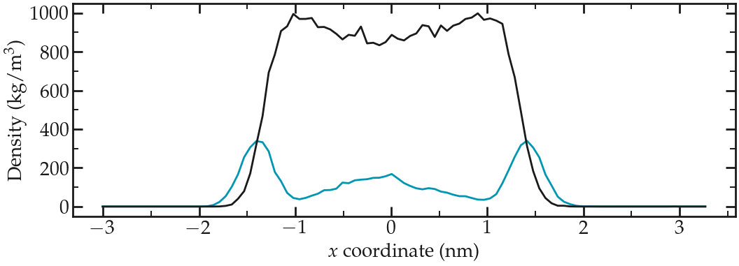
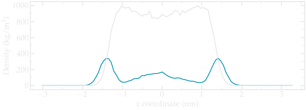
Figure: Water (blue) and ethanol (gray) density profiles along the \(x\) axis. These density profiles were obtained during the last 500 picoseconds of a 1 nanosecond long run.
The density profiles show an excess of ethanol at the 2 interfaces, which is commonly observed [28]. There is also a local maxima in the water density near the center of the fluid layer (near \(x = 3~\text{nm}\)), and two depletion areas in between the center of the fluid layer and the two interfaces.
Imposed forcing
To calculate the free energy profile across the liquid/vapor interface, one needs to impose an additional harmonic potential on one ethanol molecule and force it to explore the box along the \(x\) axis..
As a test, let us first apply the protocol to force the ethanol molecule to remain in one given single position. All the remaining positions will be calculated in the next part of this tutorial.
Within singleposition/, create a folder named inputs/, and copy min.mdp, nvt.mdp and pro.mdp in it.
In all 3 .mdp files, there are the following lines:
pull = yes
pull-nstxout = 1
pull-ncoords = 1
pull-ngroups = 2
pull-group1-name = ethanol_pull
pull-group2-name = water
pull-coord1-type = umbrella
pull-coord1-geometry = distance
pull-coord1-dim = Y N N
pull-coord1-groups = 1 2
pull-coord1-start = no
pull-coord1-init = 2
pull-coord1-rate = 0.0
pull-coord1-k = 1000
These lines specify the additional harmonic potential to be applied between a group named ethanol_pull (still to be defined) and water. The spring constant of the harmonic potential is \(k = 1000~\text{kJ/mol/nm}^2\), and the requested distance between the center-of-mass of the two groups is \(2~\text{nm}\) along the \(x\) axis.
Copy as well the previously created topol.top file within singleposition/, and modify the first lines to adapt the path to the force field folder:
#include "../preparation/ff/gromos54a7_atb.ff/forcefield.itp"
#include "../preparation/ff/BIPQ_GROMACS_G54A7FF_allatom.itp"
#include "../preparation/ff/h2o.itp"
Let us create an index file:
gmx make_ndx -f ../preparation/nvt.gro -o index.ndx
Then, type:
a 2
name 6 ethanol_pull
Press q to save and exit. These commands create an index file containing, alongside default groups, a group named ethanol_pull made of only 1 atom: the atom with index 2. This atom is the oxygen atom of the first ethanol molecule in the list.
You can ensure that the atom of index 2 is indeed an oxygen atom that beyond to an ethanol molecule by looking at the top of the nvt.gro (or nvt_1ns.gro) file:
Ethanol molecules in water
4008
    1BIPQ    H6    1   1.679   0.322   1.427 -1.2291 -2.8028 -0.6705
    1BIPQ    O1    2   1.617   0.317   1.501 -0.1421 -0.1303  0.4816
    1BIPQ    C2    3   1.549   0.441   1.496 -0.4726 -0.1734  0.4272
    1BIPQ    H4    4   1.453   0.450   1.548 -0.2059 -0.1001  0.9069
    1BIPQ    H5    5   1.529   0.454   1.390 -0.7133  0.0381  0.4988
    1BIPQ    C1    6   1.641   0.548   1.542  0.1500 -0.4454 -0.2006
    1BIPQ    H1    7   1.600   0.646   1.516  0.5688 -0.5292 -1.1624
    1BIPQ    H2    8   1.734   0.549   1.486 -1.4595  1.2268 -2.9589
    1BIPQ    H3    9   1.652   0.548   1.651 -2.4175  0.8229  0.1142
(...)
Run all 3 inputs successively using GROMACS:
gmx grompp -f inputs/min.mdp -c ../preparation/nvt_1ns.gro -p topol.top -o min -pp min -po min -maxwarn 1 -n index.ndx
gmx mdrun -v -deffnm min
gmx grompp -f inputs/nvt.mdp -c min.gro -p topol.top -o nvt -pp nvt -po nvt -maxwarn 1 -n index.ndx
gmx mdrun -v -deffnm nvt
gmx grompp -f inputs/pro.mdp -c nvt.gro -p topol.top -o pro -pp pro -po pro -maxwarn 1 -n index.ndx
gmx mdrun -v -deffnm pro
During minimization, the ethanol molecule is separated from the rest of the fluid until the distance between the center-of-mass of the 2 groups is 2 nm.
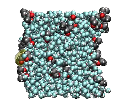
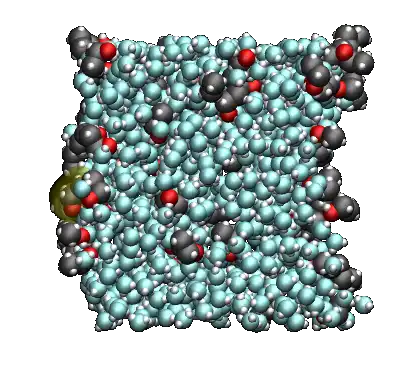
Figure: Ethanol molecule being pulled from the rest of the fluid during minimization and NVT equilibration.
Then, during the production run, the average distance between the 2 groups is measured over time.
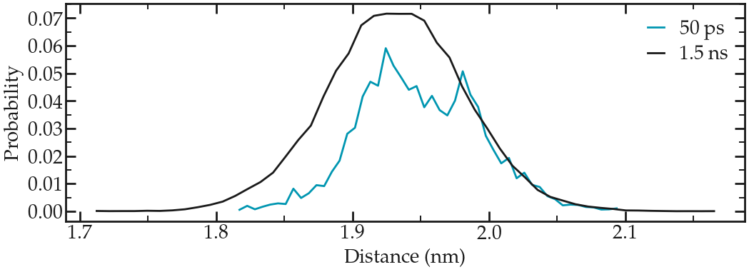
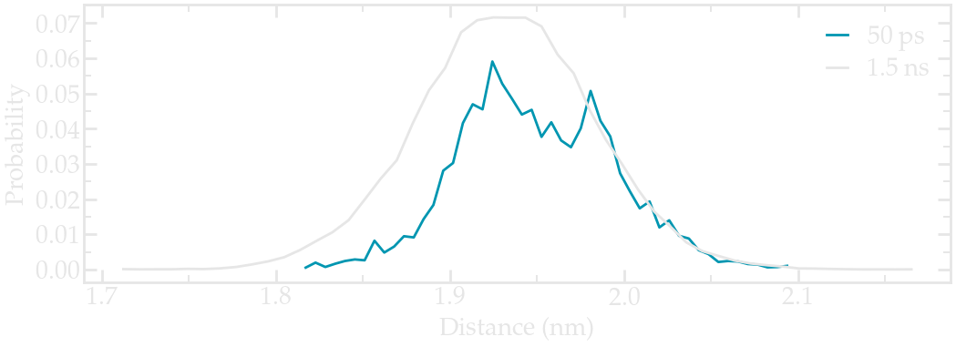
Figure: Probability distribution of the distance between the two center-of-mass. Short (50 ps) and long (1.5 ns) runs are compared.
Here, a longer run has been added for comparison. If you have the computational resources, feel free to run longer production runs than 50 ps.
Note that the distribution is not centered around \(x = 2~\text{nm}\). This is expected as the interactions between the pulled ethanol molecule and the rest of the fluid are shifting away from the average position of the ethanol molecule from the center of harmonic potential.
Free energy profile calculation
Let us replicate the previous calculation for 30 distances, from \(x = 0\) (i.e. the center of the liquid slab) to \(x = 4~\text{nm}\) (far within the vacuum phase). Within the folder called adsorption/, create an inputs/ folder, and copy min.mdp, nvt.mdp, and pro.mdp, in it.
The only difference with the previous input scripts is the command:
pull-coord1-init = to_be_replaced
Here, the keyword to_be_replaced is to be systematically replaced by the right number using the bash script below.
Create a new bash script called run.sh with adsorption/, and copy the following lines in it:
#!/bin/bash

set -e

for ((i = 0 ; i < 30 ; i++)); do
        x=$(echo "0.13*$(($i+1))" | bc);
        sed 's/to_be_replaced/'$x'/g' inputs/min.mdp > min.mdp
        gmx grompp -f min.mdp -c ../preparation/nvt_1ns.gro -p topol.top -o min.$i -pp min.$i -po min.$i -maxwarn 1 -n index.ndx
        gmx mdrun -v -deffnm min.$i

        sed 's/to_be_replaced/'$x'/g' inputs/nvt.mdp > nvt.mdp
        gmx grompp -f nvt.mdp -c min.$i.gro -p topol.top -o nvt.$i -pp nvt.$i -po nvt.$i -maxwarn 1 -n index.ndx
        gmx mdrun -v -deffnm nvt.$i

        sed 's/to_be_replaced/'$x'/g' inputs/pull.mdp > pull.mdp
        gmx grompp -f pull.mdp -c nvt.$i.gro -p topol.top -o pull.$i -pp pull.$i -po pull.$i -maxwarn 1 -n index.ndx
        gmx mdrun -v -deffnm pull.$i
done
Copy the previously created index file and topology file within the adsorption/ folder, and execute the bash script.
When the simulation is done, create 2 files by typing in the terminal (credit to the gaseri site):
ls prd.*.tpr > tpr.dat
ls pullf-prd.*.xvg > pullf.dat
Finally, perform the analysis using the gmx wham command of GROMACS:
gmx wham -it tpr.dat -if pullf.dat
A file named profile.xvg has been created. It contains a potential of mean force (PMF).
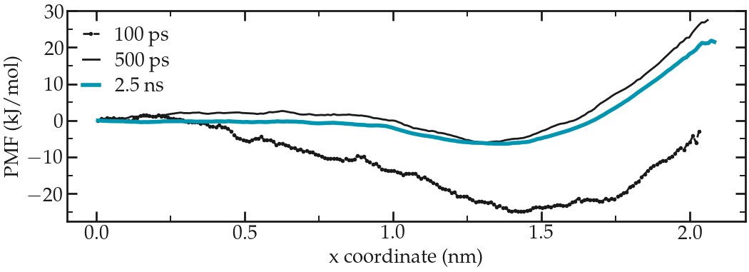
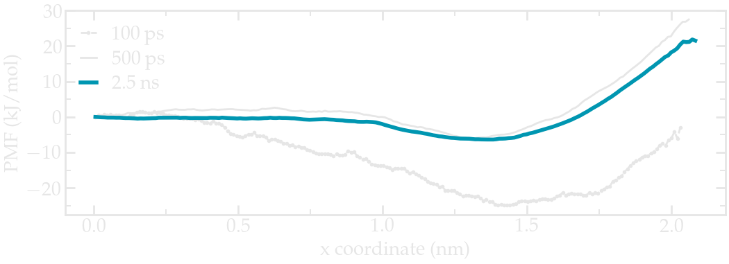
Figure: PMF for the ethanol molecule across the interface between a water/ethanol liquid slab and vapor.
The durations of 100 ps used in this tutorial are too short to obtain a smooth and reliable PMF curve. Increase the duration of the production runs to a few nanoseconds for reasonable results.
The PMF shows a plateau inside the bulk liquid (\(x<1~\text{nm}\)), a minimum at the interface (\(x=1.5~\text{nm}\)), and increase in the vapor phase (\(x>1.5~\text{nm}\)). The minimum at the interface indicate that ethanol favorably adsorb at the liquid/vapor interface, which is consistent with the density profile.
The PMF also indicates that once adsorbed, the ethanol molecule requires an energy of about \(5~\text{kJ/mol}\) to re-enter the liquid phase (see blue curve), which is about \(2.2~k_\text{B} T\).
Finally, the PMF shows that it is energetically costly for the ethanol molecule to fully desorb and go into the vacuum phase as the energy barrier to overcome is at least \(25~\text{kJ/mol}\). Consistently, when performing unbiased MD simulation, it is relatively rare to observe an ethanol molecule exploring the vapor phase.
You can access all the input scripts and data files that are used in these tutorials from |GitHub-repository|.