Stretching a polymer

Solvating and stretching a small polymer molecule

The goal of this tutorial is to use GROMACS and solvate a small hydrophilic polymer in a reservoir of water.

An all-atom description is used for both polymer and water. The polymer is PolyEthylene Glycol (PEG). Once the system is properly equilibrated at the desired temperature and pressure, a force is applied to both ends of the polymer. The evolution of the polymer length is measured, and the energetics of the system is analyzed. This tutorial is inspired by a publication by Susanne Liese and coworkers, in which molecular dynamics simulations are compared with force spectroscopy experiments [24].

If you are completely new to GROMACS, I recommend that you follow this tutorial on a simple bulk-solution-label first.

Struggling with your molecular simulations project?

Get guidance for your GROMACS simulations. contact-label for personalized advice for your project.

This tutorial is compatible with the 2024.2 GROMACS version.

Prepare the PEG molecule

Download the peg.gro file for the PEG molecule by clicking. The peg.gro file can be visualized using VMD, by typing in a terminal:

vmd peg.gro

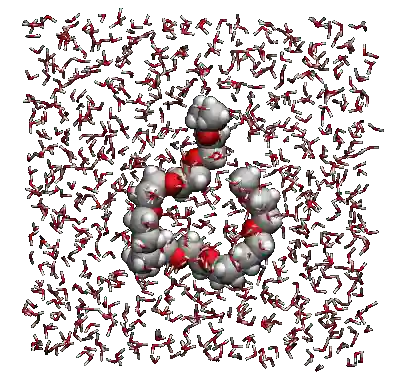
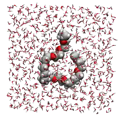
Figure: The PEG molecule is a polymer chain made of carbon atoms (in gray), oxygen atoms (in red), and hydrogen atoms (in white). See the corresponding video.

Save peg.gro in a new folder. Next to peg.gro create an empty file named topol.top, and copy the following lines into it:

[ defaults ]
; nbfunc    comb-rule    gen-pairs    fudgeLJ    fudgeQQ
    1         1            no           1.0     1.0

; Include forcefield parameters
#include "ff/charmm35r.itp"
#include "ff/peg.itp"
#include "ff/tip3p.itp"

[ system ]
; Name
    PEG

[ molecules ]
; Compound        #mols
    PEG             1

Next to conf.gro and topol.top, create a folder named ff/, and copy the following 3 .itp files into it: charmm35r.itp, peg.itp, and tip3p.itp. These files provide the necessary force field parameters for both the PEG (C, OE, H, OT, and HT atoms) and the water molecules (OW and HW atoms).

Note

The charmm35r.itp file contains the atomic masses, partial charges, and Lennard-Jones nonbonded interaction parameters. The peg.itp and tip3p.itp files define the bonded parameters for PEG and water molecules, including bonds, angles, and dihedrals contraints.

Create an inputs/ folder next to ff/, and create a new empty file called em.mdp into it. Copy the following lines into em.mdp:

integrator = steep
emtol = 10
emstep = 0.0001
nsteps = 5000

nstenergy = 1000
nstxout = 100

cutoff-scheme = Verlet
coulombtype = PME
rcoulomb = 1
rvdw = 1
pbc = xyz

Most of these commands have been seen in previous tutorials. Arguably the most important command is integrator = steep, which sets the algorithm used by GROMACS as the steepest-descent method. This algorithm moves the atoms following the direction of the largest forces until one of the stopping criteria is reached [13]. The stopping criteria include reaching the maximum force tolerance set by emtol, or completing the maximum number of steps specified by nsteps. The initial step size for energy minimization is controlled by emstep. Other parameters define the treatment of nonbonded interactions, such as cutoff-scheme = Verlet, electrostatics handled by Particle-Mesh Ewald with coulombtype = PME, cutoff distances rcoulomb and rvdw set to 1 nm. Periodic boundary conditions are applied in all directions with pbc = xyz. Output frequencies for energy and coordinate writing are set by nstenergy and nstxout, respectively.

Run the energy minimization using GROMACS by typing in a terminal:

gmx grompp -f inputs/em.mdp -c peg.gro -p topol.top -o em-peg
gmx mdrun -deffnm em-peg -v -nt 8

The -nt 8 option limits the number of threads that GROMACS uses. Adjust the number to your computer.

After the simulation is complete, open the trajectory file with VMD by typing the following command in a terminal:

vmd peg.gro em-peg.trr

In VMD, you can observe the PEG molecule moving slightly as a result of the steepest-descent energy minimization.

Before adding water, let us reshape the box and recenter the PEG molecule within it. Let us also place it in a cubic box with a lateral size of \(2.6~\text{nm}\).

gmx trjconv -f em-peg.gro -s em-peg.tpr -o peg-recentered.gro -center
-pbc mol -box 2.6 2.6 2.6

Select system for both the centering and output prompts. The newly created peg-recentered.gro file will be used as the starting point for the next step of the tutorial.

Solvate the PEG molecule

Let us add water molecules to the system using gmx solvate:

gmx solvate -cp peg-recentered.gro -cs spc216.gro -o peg-solvated.gro -p topol.top

Here, spc216.gro is a default GROMACS file containing a pre-equilibrated water reservoir. The newly created file peg-solvated.gro contains the water molecules, and a new line has been added to the topology file topol.top:

[ molecules ]
; Compound        #mols
PEG               1
SOL               546

We can apply the same energy minimization as before to the newly created solvated system. Simply add the following line to em.mdp:

define = -DFLEXIBLE

With the define = -DFLEXIBLE option, the water molecules are treated as flexible during energy minimization, enabling bond stretching and angle bending in water. The define = -DFLEXIBLE option triggers the following if condition within the tip3p.itp file:

#ifdef FLEXIBLE
[ bonds ]
; i     j       funct   length  force.c.
1       2       1       0.09572 502416.0 0.09572        502416.0
1       3       1       0.09572 502416.0 0.09572        502416.0

[ angles ]
; i      j      k       funct   angle   force.c.
2        1      3       1       104.52  628.02  104.52  628.02

With this if condition, the water molecules behave as flexible, which is preferable because rigid molecules and energy minimization usually do not work well together.

Note

For the subsequent molecular dynamics steps, rigid water molecules will be used by removing the define = -DFLEXIBLE command from the inputs.

Finally, launch the energy minimization again using:

gmx grompp -f inputs/em.mdp -c peg-solvated.gro -p topol.top -o em
gmx mdrun -deffnm em -v -nt 8

Equilibrate the PEG-water system

Let us further equilibrate the system in two steps: first, an NVT simulation with constant number of particles, constant volume, and imposed temperature; and second, an NpT simulation with imposed pressure. Within the inputs/ folder, create a new input file named nvt-peg-h2o.mdp, and copy the following lines into it:

integrator = md
dt = 0.002
nsteps = 10000

nstenergy = 500
nstlog = 500
nstxout-compressed = 500

constraint-algorithm = lincs
constraints = hbonds
continuation = no

coulombtype = pme
rcoulomb = 1.0
rlist = 1.0

vdwtype = Cut-off
rvdw = 1.0

tcoupl = v-rescale
tau_t = 0.1 0.1
ref_t = 300 300
tc_grps = PEG Water

gen-vel = yes
gen-temp = 300
gen-seed = 65823

comm-mode = linear
comm-grps = PEG

Most of these commands have already been seen. In addition to the conventional md leap-frog algorithm integrator, with long-range Coulomb and short-range van der Waals interactions, the LINCS constraint algorithm is used to keep the hydrogen bonds rigid. Temperature coupling at \(300~K\) is imposed on both the PEG and water groups using velocity rescaling with a stochastic term (tcoupl = v-rescale). Initial velocities at \(300~K\) are generated by the gen- commands, with a specified random seed. The comm-mode and comm-grps commands ensure that the PEG molecule remains centered in the box by removing its center-of-mass motion separately from the solvent.

Launch the NVT simulation using:

gmx grompp -f inputs/nvt-peg-h2o.mdp -c em.gro -p topol.top -o nvt -maxwarn 1
gmx mdrun -deffnm nvt -v -nt 8

The -maxwarn 1 option is used to bypass a GROMACS warning related to the centering of the PEG molecule in the box.

Let us follow up with the NPT equilibration. Duplicate the nvt-peg-h2o.mdp file into a new input file named npt-peg-h2o.mdp. Within npt-peg-h2o.mdp, delete the lines related to the creation of velocities, as it is better to preserve the velocities generated during the previous NVT run:

gen_vel = yes
gen-temp = 300
gen-seed = 65823

In addition to removing these three lines, add the following lines to npt-peg-h2o.mdp to enable an isotropic barostat with an imposed pressure of \(1~\text{bar}\):

pcoupl = c-rescale
pcoupltype = isotropic
tau-p = 0.5
ref-p = 1.0
compressibility = 4.5e-5

These last five lines configure the pressure coupling. The pcoupl option selects the c-rescale barostat, a stochastic barostat suitable for equilibration. The pressure coupling type is set to isotropic, meaning the box dimensions scale uniformly in all directions. The tau-p parameter defines the coupling time constant in picoseconds, determining how quickly the system adjusts to the target pressure. The ref-p sets the reference pressure at \(1~\text{bar}\), and compressibility specifies the isothermal compressibility of water, which is required for volume fluctuations to properly reflect the solvent properties.

Run the NpT simulation, using the final state of the NVT simulation nvt.gro as starting configuration:

${gmx} grompp -f inputs/npt-peg-h2o.mdp -c nvt.gro -p topol.top -o npt -maxwarn 1
${gmx} mdrun -deffnm npt -v -nt 8

Let us observe the evolution of the potential energy of the system during the three successive equilibration steps, i.e. the energy minimization, NVT, and NpT steps, using the gmx energy command as follows:

gmx energy -f em.edr -o energy-em.xvg
gmx energy -f nvt.edr -o energy-nvt.xvg
gmx energy -f npt.edr -o energy-npt.xvg

For each of the three gmx energy commands, select Potential when prompted.

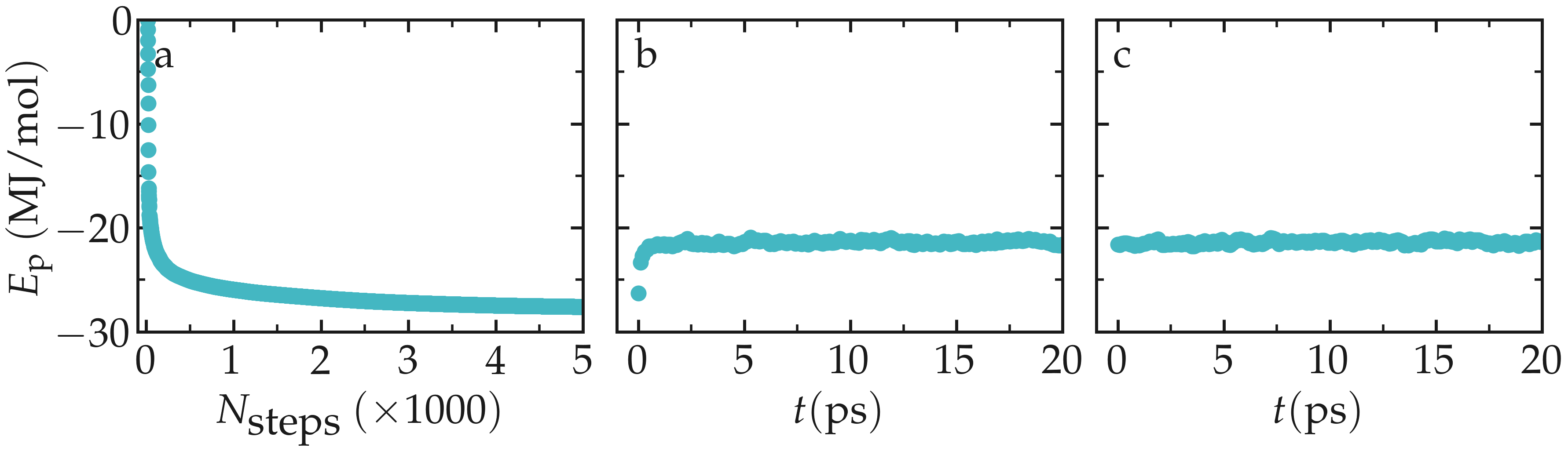
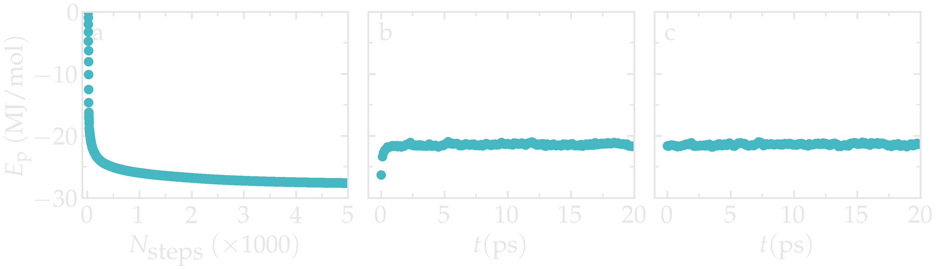
Figure: Evolution of the potential energy during the 3 equilibration steps, respectively the energy minimization (a), the NVT step (b), and the NPT step (c).

Let us launch a longer simulation and extract the angle distribution between the different atoms of the PEG molecule. This angle distribution will later serve as a benchmark to assess the effect of stretching on the PEG structure. Create a new input file named production-peg-h2o.mdp, and copy the following lines into it:

integrator = md
dt = 0.002
nsteps = 50000

nstenergy = 100
nstlog = 100
nstxout-compressed = 100

constraint-algorithm = lincs
constraints = hbonds
continuation = no

coulombtype = pme
rcoulomb = 1.0
rlist = 1.0

vdwtype = Cut-off
rvdw = 1.0

tcoupl = v-rescale
tau_t = 0.1 0.1
ref_t = 300 300
tc_grps = PEG Water

comm-mode = linear
comm-grps = PEG

This input file is similar to nvt-peg-h2o.mdp, but with a longer simulation time and more frequent output, and without the gen-vel commands to preserve the velocities from the previous equilibration.

Run it using:

gmx grompp -f inputs/production-peg-h2o.mdp -c npt.gro -p topol.top -o production -maxwarn 1
gmx mdrun -deffnm production -v -nt 8

First, create an index file called angle.ndx using the gmx mk_angndx command:

gmx mk_angndx -s production.tpr -hyd no

The angle.ndx file generated contains groups of all atoms involved in angle constraints, with hydrogen atoms excluded thanks to the -hyd no option. The atom indices included in the groups can be verified in the index.ndx file:

[ Theta=109.7_795.49 ]
    2     5     7    10    12    14    17    19    21    24    26    28
    31    33    35    38    40    42    45    47    49    52    54    56
    59    61    63    66    68    70    73    75    77    80    82    84

Here, each number corresponds to an atom index, as listed in the initial peg.gro file. For example, atom id 2 is a carbon atom, and atom id 5 is an oxygen atom:

PEG in water
86
    1PEG      H    1   2.032   1.593   1.545  0.6568  2.5734  1.2192
    1PEG      C    2   1.929   1.614   1.508  0.1558 -0.2184  0.8547
    1PEG     H1    3   1.902   1.721   1.523 -3.6848 -0.3932 -3.0658
    1PEG     H2    4   1.921   1.588   1.400 -1.5891  1.4960  0.5057
    1PEG      O    5   1.831   1.544   1.576  0.0564 -0.5300 -0.6094
    1PEG     H3    6   1.676   1.665   1.494 -2.6585 -0.5997  0.3128
    1PEG     C1    7   1.699   1.559   1.519  0.6996  0.0066  0.2900
    1PEG     H4    8   1.699   1.500   1.425  4.2893  1.6837 -0.9462
(...)

Then, extract the angle distribution from the production.xtc trajectory using gmx angle:

gmx angle -n angle.ndx  -f production.xtc -od angle-distribution.xvg -binwidth 0.25

When prompted, select group 1 corresponding to the O-C-C-O dihedral.

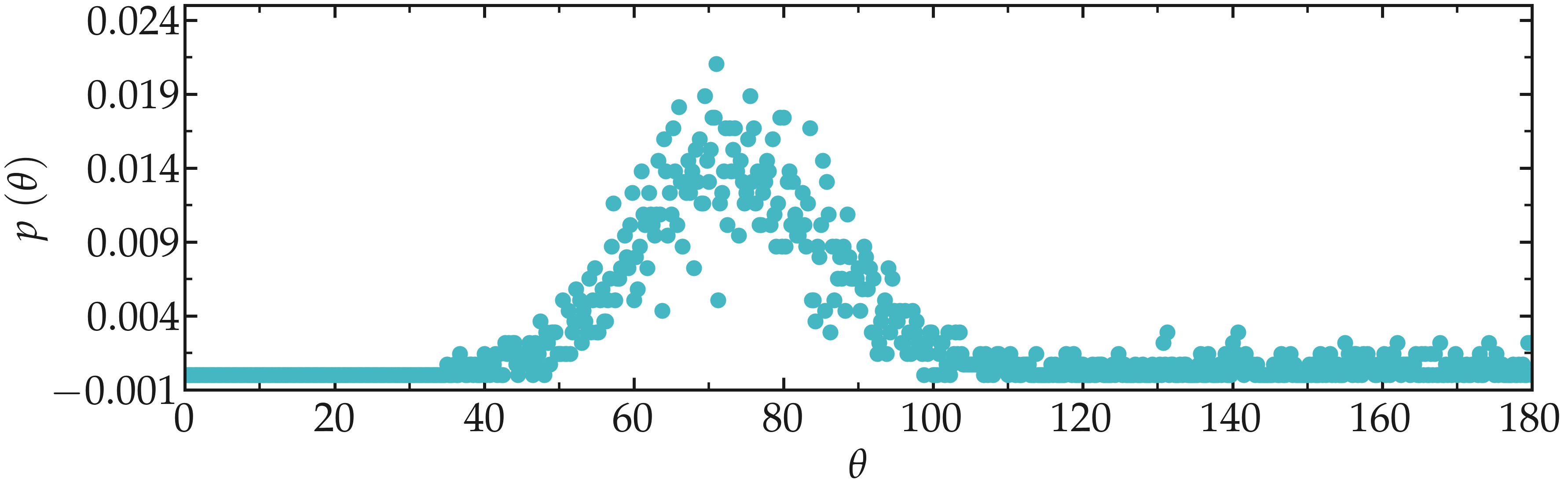
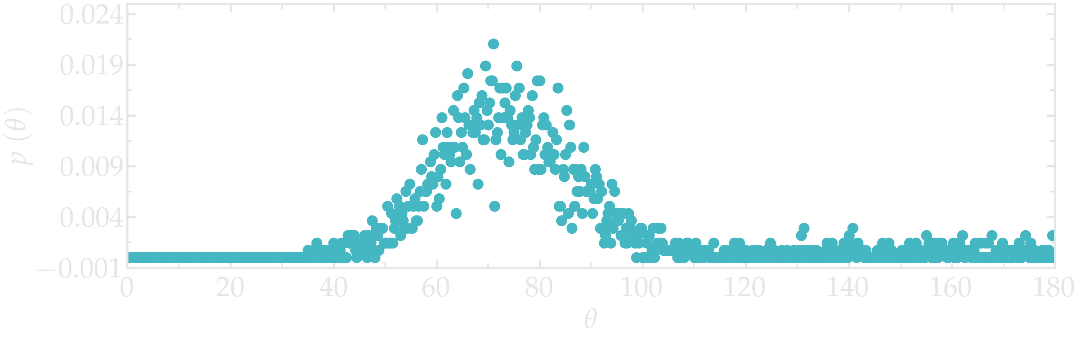
Figure: Angular distribution for the O-C-C-O dihedral of the PEG molecules.

Stretch on the polymer

Create a new folder named elongated-box/ next to cubic-box/, and copy ff/, inputs/, em-peg.gro, and em-peg.tpr from cubic-box/ into elongated-box/:

To leave space for the stretched PEG molecule, let us create an elongated box of length \(6~\text{nm}\) along the x direction:

gmx trjconv -f em-peg.gro -s em-peg.tpr -o peg-elongated.gro -center -pbc mol -box 6 2.6 2.6

Select system for both centering and output.

Then, follow the exact same steps as previously to solvate and equilibrate the system:

gmx solvate -cp peg-elongated.gro -cs spc216.gro -o peg-solvated.gro -p topol.top

gmx grompp -f inputs/em.mdp -c peg-solvated.gro -p topol.top -o em -maxwarn 1
gmx mdrun -deffnm em -v -nt 8

gmx grompp -f inputs/nvt-peg-h2o.mdp -c em.gro -p topol.top -o nvt -maxwarn 1
gmx mdrun -deffnm nvt -v -nt 8

gmx grompp -f inputs/npt-peg-h2o.mdp -c nvt.gro -p topol.top -o npt -maxwarn 1
gmx mdrun -deffnm npt -v -nt 8

The index file

To apply a forcing to the ends of the PEG, one needs to create atom groups. Specificaly, we want to create two groups, each containing a single oxygen atom from the edges of the PEG molecules (with id 82 and 5). In GROMACS, this can be done using and index file .ndx. Create a new index file named index.ndx using the gmx make_ndx command:

gmx make_ndx -f nvt.gro -o index.ndx

When prompted, type the following 4 lines to create 2 additional groups:

a 82
a 5
name 6 End1
name 7 End2

Then, type q for quitting. The index file index.ndx contains 2 additional groups named End1 and End2:

(...)
[ PEG ]
1    2    3    4    5    6    7    8    9   10   11   12   13   14   15
16   17   18   19   20   21   22   23   24   25   26   27   28   29   30
31   32   33   34   35   36   37   38   39   40   41   42   43   44   45
46   47   48   49   50   51   52   53   54   55   56   57   58   59   60
61   62   63   64   65   66   67   68   69   70   71   72   73   74   75
76   77   78   79   80   81   82   83   84   85   86
[ End1 ]
82
[ End2 ]
5

The input file

Let us create an input file for the stretching of the PEG molecule.

Create a new input file named stretching-peg-h2o.mdp within inputs/, and copy the following lines in it:

integrator = md
dt = 0.002
nsteps = 50000

nstenergy = 100
nstlog = 100
nstxout-compressed = 100

constraint-algorithm = lincs
constraints = hbonds
continuation = no

coulombtype = pme
rcoulomb = 1.0
rlist = 1.0

vdwtype = Cut-off
rvdw = 1.0

tcoupl = v-rescale
tau_t = 0.1 0.1
ref_t = 300 300
tc_grps = PEG Water

So far, the script is similar to the previously created production-peg-h2o.mdp file, but without the comm-mode commands. To apply the constant forcing to the End1 and End2 groups, add the following lines to production-peg-h2o.mdp:

pull = yes
pull-coord1-type = constant-force
pull-ncoords = 1
pull-ngroups = 2
pull-group1-name = End1
pull-group2-name = End2
pull-coord1-groups = 1 2
pull-coord1-geometry = direction-periodic
pull-coord1-dim = Y N N
pull-coord1-vec = 1 0 0
pull-coord1-k = 200
pull-coord1-start = yes
pull-print-com = yes

The force constant is requested along the x direction only (Y N N), with a force constant \(k = 200~\text{kJ}~\text{mol}^{-1}~\text{nm}^{-1}\).

Launch the simulation using the -n index.ndx option for the gmx grompp command to refer to the previously created index file, so that GROMACS finds the End1 and End2 groups.

gmx grompp -f inputs/stretching-peg-h2o.mdp -c npt.gro -p topol.top -o stretching -n index.ndx
gmx mdrun -deffnm stretching -v -nt 8

Two data files named stretching_pullf.xvg and stretching_pullx.xvg are created during the simulation, and contain respectively the force and distance between the 2 groups End1 and End2 as a function of time.

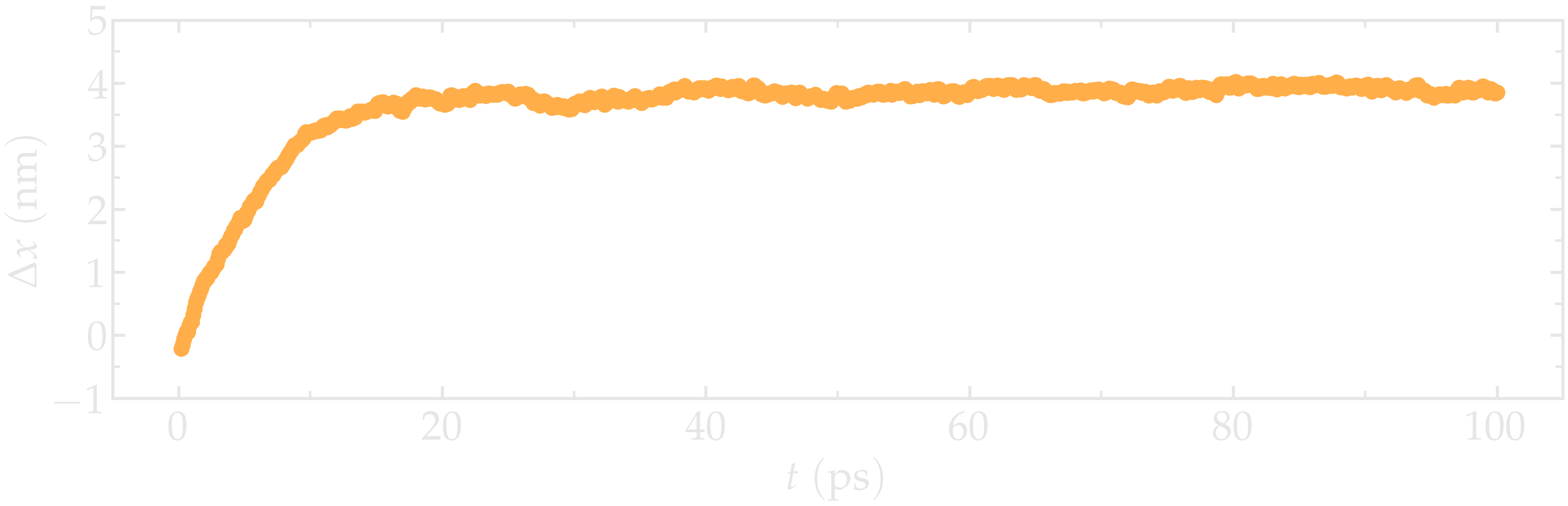
Figure: Distance between the two pulled groups End1 and End2 along the x direction, \(\Delta x\), as a function of time \(t\).

It can be seen from the evolution of the distance between the groups, \(\Delta x\), that the system reaches its equilibrium state after approximately 20 pico-seconds.

Let us probe the effect of the stretching on the structure of the PEG by remeasuring the dihedral angle values:

gmx mk_angndx -s stretching.tpr -hyd no -type dihedral
gmx angle -n angle.ndx  -f stretching-centered.xtc -od dihedral-distribution.xvg -binwidth 0.25 -type dihedral -b 20

Select 1 for the O-C-C-O dihedral. Here, the option -b 20 is used to disregard the first 20 pico-seconds of the simulation during which the PEG has not reach is final length.

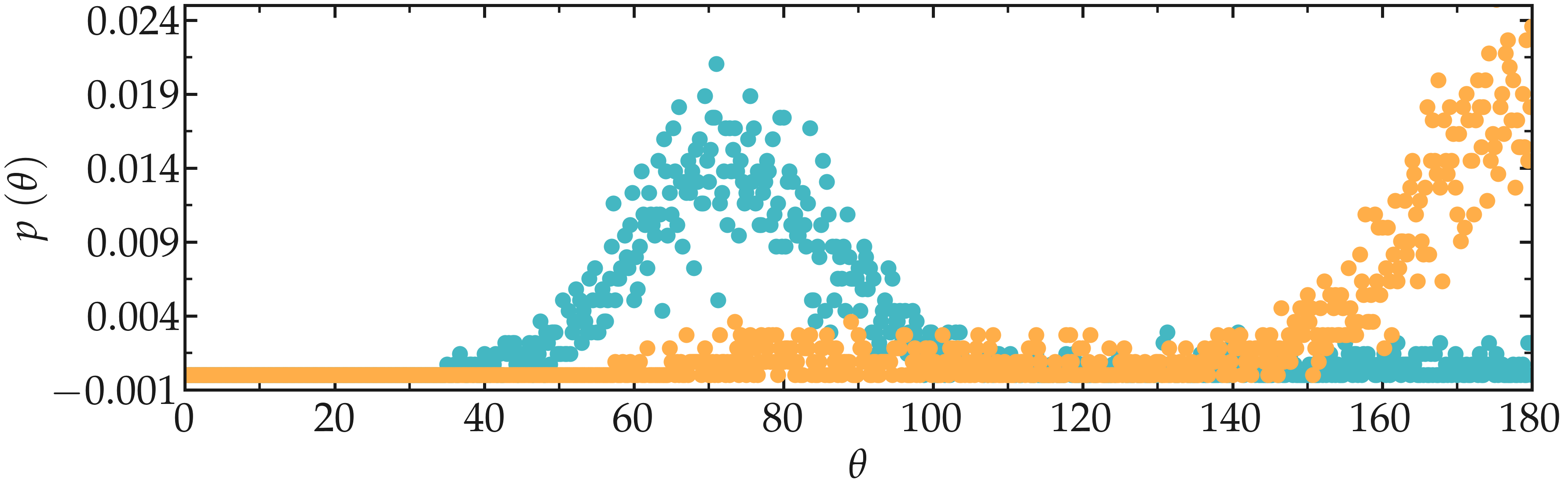
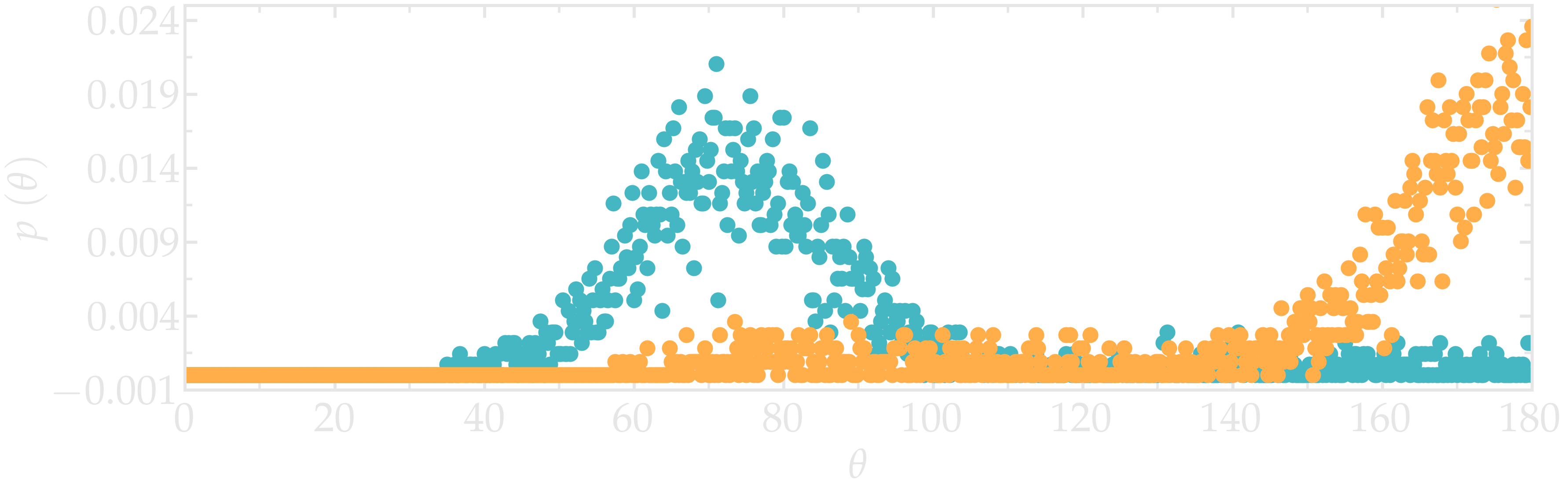
Figure: Angular distribution for the O-C-C-O dihedral of the PEG molecules, comparing the unstretched (cyan) and stretched case (orange).

The change in dihedral angles disribution reveals a configurational change of the polymer induced by the forcing. This transition is called gauche-trans, where gauche and trans refer to possible states for the PEG monomer [24, 25].

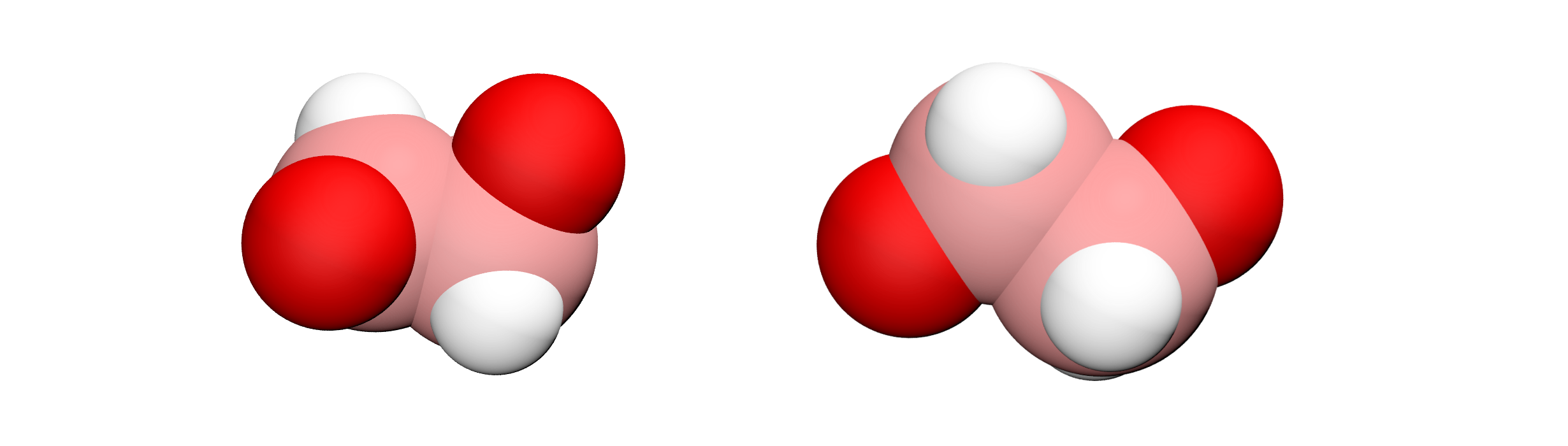
Figure: Illustration of the gauche (left) and trans (right) states of the PEG polymer.

You can access all the input scripts and data files that are used in these tutorials from GitHub.