Molecule solvation energy#
Free energy solvation calculation of a disk-like molecule
The objective of this tutorial is to use GROMACS to perform a molecular dynamics simulation, and to calculate the free energy of solvation of a large molecule in water.
The large molecule used here is a graphene-like and disk-like molecule named hexabenzocoronene.
If you are completely new to GROMACS, I recommend you to follow this simpler tutorial first : Bulk salt solution.
Looking for help with your project?
See the Contact page.
Input files#
Create two folders named ‘preparation/’ and ‘solvation’ in the same directory, and go to ‘preparation/’.
Download the configuration files for the HBC molecule by clicking here (its from the atb), and place it in the ‘preparation/’ folder.
Create the configuration file#
First, let us convert the pdb file into a gro file within a box of finite size (4 nm by 4 nm by 4 nm) using trj conv:
gmx trjconv -f FJEW_allatom_optimised_geometry.pdb -s FJEW_allatom_optimised_geometry.pdb -o hbc.gro -box 4 4 4 -center
Select ‘system’ for both centering and output.
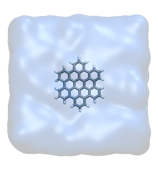
If you open the hbc.gro file with VMD, you will see:


HBC molecule with carbon atoms in gray and hydrogen atoms in white. The honey-comb structure of HBC is similar to that of graphene.#
Alternatively, you can download the file I have generated and continue with the tutorial.
Create the topology file#
Copy the force field files (ITP file)in a folder named ‘ff/’ and located within the ‘preparation/’ folder. Force field parameters can be downloaded as a zip file by clicking here.
All the files contained in the ff folder were downloaded from the atb.
Then, let us write the topology file by simply creating a blank file named ‘topol.top’ within the ‘preparation/’ folder, and copying in it:
#include "ff/gromos54a7_atb.ff/forcefield.itp"
#include "ff/FJEW_GROMACS_G54A7FF_allatom.itp"

[ system ]
Single HBC molecule

[ molecules ]
FJEW 1
Add the water#
Let us add water molecules to the system. First, download the tip4p water configuration file here, and copy it in the ‘preparation/’ folder. Then, in order to add (tip4p) water molecules to both gro and top file, use the gmx solvate command as follow:
gmx solvate -cs tip4p.gro -cp hbc.gro -o solvated.gro -p topol.top
You should see the following message:
Processing topology
Adding line for 2186 solvent molecules with resname (SOL) to topology file (topol.top)
and a new line ‘SOL 2186’ in the topology file:
[ molecules ]
FJEW 1
SOL 2186
The created ‘solvated.gro’ file contains the positions of both HBC (called FJEW) and water molecules . Alternatively, you can download the file I have generated by clicking here.
The only missing information is the force field for the water molecule. In order to use the TIP4P/epsilon water model, which is one of the best classical water model, copy the h2o.itp file in the ‘ff/’ folder and modify the beginning of the topology file as follow:
#include "ff/gromos54a7_atb.ff/forcefield.itp"
#include "ff/FJEW_GROMACS_G54A7FF_allatom.itp"
#include "ff/h2o.itp"
The system is ready, let us equilibrate it before measuring the solvation energy of the HBC molecule.
Energy minimization#
Create a new folder in the preparation/’ folder, call it ‘inputs’, and save a new blank file, called min.mdp, in it. Copy the following lines into min.mdp:
integrator = steep
nsteps = 50

nstxout = 10

cutoff-scheme = Verlet
nstlist = 10
ns_type = grid

couple-intramol=yes

vdw-type = Cut-off
rvdw = 1.2

coulombtype = pme
fourierspacing = 0.1
pme-order = 4
rcoulomb = 1.2

constraint-algorithm = lincs
constraints = hbonds
All these lines have been seen in the first tutorial (Bulk salt solution). In short, this script will perform a steepest descent by updating the atom positions according to the largest forces directions, until the energy and maximum force reach a reasonable value.
Apply the minimisation to the solvated box using:
gmx grompp -f inputs/min.mdp -c solvated.gro -p topol.top -o min -pp min -po min -maxwarn 1
gmx mdrun -v -deffnm min
Here the ‘-maxwarn 1’ allows us to perform the simulation despite GROMACS’ warning about some force field issue. Since this is a tutorial and not actual research, we can safely ignore this warning.
Let us visualize the atoms’ trajectories during the minimization step using VMD by typing:
vmd solvate.gro min.trr
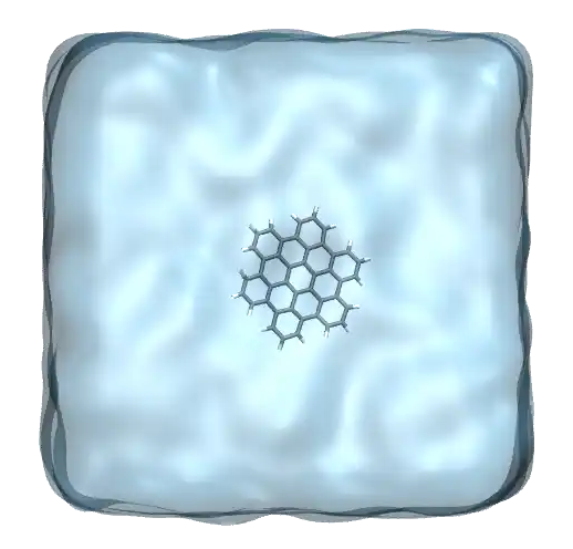
The final state looks like that:


HBC molecule in water after energy minimization. Water is represented as a transparent field.#
Equilibration#
Let us perform successively a NVT and a NPT relaxation. Copy the nvt.mdp and the npt.mdp files into the inputs folder, and run them both using:
gmx grompp -f inputs/nvt.mdp -c min.gro -p topol.top -o nvt -pp nvt -po nvt -maxwarn 1
gmx mdrun -v -deffnm nvt
gmx grompp -f inputs/npt.mdp -c nvt.gro -p topol.top -o npt -pp npt -po npt -maxwarn 1
gmx mdrun -v -deffnm npt
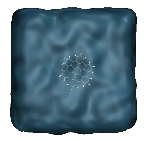
The simulation looks like that:
Movie showing the motion of the atoms during the NVT and NPT equilibration steps. For clarity, the water molecules are represented as a continuum field.#
Here we use maxwarn 1 to disregard a GROMACS warning about the force field. If you want to publish your research, don’t ignore that warning lightly.
Support me for 1 euro per month
Become a Patreon and support the creation of content for GROMACS
Solvation energy measurement#
We are done with the first equilibration of the system. We are now going to perform the solvation free energy calculation, for which 21 independent simulations will be performed.
Quick explanation of the procedure: The interactions between the HBC molecule and water are progressively turned-off, thus effectively mimicking the HBC molecule moving from bulk water to vacuum.
Within the ‘solvation/’ folder, create an ‘inputs/’ folders. Copy the two following npt_bis.mdp and pro.mdp files in it.
Both files contain the following commands that are related to the free energy calculation:
free_energy = yes
vdw-lambdas = 0.0 0.1 0.2 0.3 0.4 0.5 0.6 0.7 0.8 0.9 1.0 1.0 1.0 1.0 1.0 1.0 1.0 1.0 1.0 1.0 1.0
coul-lambdas = 0.0 0.0 0.0 0.0 0.0 0.0 0.0 0.0 0.0 0.0 0.0 0.1 0.2 0.3 0.4 0.5 0.6 0.7 0.8 0.9 1.0
sc-alpha = 0.5
sc-power = 1
init-lambda-state =  0
couple-lambda0 = none
couple-lambda1 = vdw-q
nstdhdl = 100
calc_lambda_neighbors = -1
couple-moltype = FJEW
These lines specify that the decoupling between the molecule of interest (here FJEW) and the rest of the system (here water) must be done by progressively turning off van der Waals and Coulomb interactions. The parameter nstdhdl controls the frequency at which information are being printed in a xvg file during the production run.
In addition, the stochastic integrator ‘sd’ is used instead of ‘md’, as it provides a better sampling, which is crucial here, particularly when the HBC and the water molecules are not coupled.
Copy as well the following topol.top file within the ‘solvation/’ folder (the only difference with the previous one if the path to the ff folder).
We need to create 21 folders, each containing the input files with different value of init-lambda-state (from 0 to 21). To do so, create a new bash file fine within the ‘solvation/’ folder, call it ‘createfolders.sh’ can copy the following lines in it:
#/bin/bash
# delete runall.sh if it exist, then re-create it
if test -f "runall.sh"; then
    rm runall.sh
fi
touch runall.sh
echo '#/bin/bash' >> runall.sh
echo '' >> runall.sh
# folder for analysis
mkdir -p dhdl
# loop on the 21 lambda state
for state in $(seq 0 20);
do
    # create folder
    DIRNAME=lambdastate${state}
    mkdir -p $DIRNAME
    # copy the topology, inputs, and configuration file in the folder
    cp -r topol.top $DIRNAME
    cp -r ../preparation/npt.gro $DIRNAME/preparedstate.gro
    cp -r inputs $DIRNAME
    # replace the lambda state in both npt_bis and production mdp file
    newline='init-lambda-state = '$state
    linetoreplace=$(cat $DIRNAME/inputs/npt_bis.mdp | grep init-lambda-state)
    sed -i '/'"$linetoreplace"'/c\'"$newline" $DIRNAME/inputs/npt_bis.mdp
    sed -i '/'"$linetoreplace"'/c\'"$newline" $DIRNAME/inputs/pro.mdp
    # create a bash file to launch all the simulations
    echo 'cd '$DIRNAME >> runall.sh
    echo 'gmx grompp -f inputs/npt_bis.mdp -c preparedstate.gro -p topol.top -o npt_bis -pp npt_bis -po npt_bis -maxwarn 1' >> runall.sh
    echo 'gmx mdrun -v -deffnm npt_bis -nt 4' >> runall.sh
    echo 'gmx grompp -f inputs/pro.mdp -c npt_bis.gro -p topol.top -o pro -pp pro -po pro -maxwarn 1' >> runall.sh
    echo 'gmx mdrun -v -deffnm pro -nt 4' >> runall.sh
    echo 'cd ..' >> runall.sh
    echo '' >> runall.sh
    # create links for the analysis
    cd dhdl
    ln -sf ../$DIRNAME/pro.xvg md$state.xvg
    cd ..
done
Change the ‘-nt 4’ to use a different number of thread if necessary.
Execute the bash script by typing:
bash createfolders.sh
The bash file creates 21 folders, each containing the input files with init-lambda-state from 0 to 21, as well as a ‘topol.top’ file and a ‘preparedstate.gro’ corresponding to the last state of the system simulated in the ‘preparation/’ folder. Run all 21 simulations by executing the ‘runall.sh’ script:
bash runall.sh
This may take a while, depending on your computer.
When the simulation is complete, go the dhdl folder, and type:
gmx bar -f *.xvg
The value of the solvation energy is printed in the terminal:
total 0 - 20, DG -37.0 +/- 8.40
The present simulations are too short to give a proper result. To actually measure the solvation energy of a molecule, use much longer equilibration (typically one nanosecond) and production runs (typically several nanoseconds).
Contact me
Contact me if you have any question or suggestion about these tutorials.