Bulk salt solution#
The very basics of GROMACS through a simple example
The objective of this tutorial is to use the open-source code GROMACS to perform a simple molecular dynamics simulation: a liquid solution of water mixed with sodium (Na+) and sulfate (SO42-) ions.
This tutorial illustrates several major ingredients of molecular dynamics simulations, such as energy minimization, thermostating, NVT and NPT equilibration, and trajectory visualisation.
There are no prerequisite to follow this tutorial.
Looking for help with your project?
See the Contact page.
Required softwares#
GROMACS must be installed on your machine. You can install it following the instructions of the GROMACS manual.
Alternatively, if you are using Ubuntu OS, you can simply execute the following command in a terminal:
sudo apt-get install gromacs
You can verify that GROMACS is indeed installed on your computer by typing in a terminal :
gmx
You should see the version of GROMACS that has been installed. On my computer I see
:-) GROMACS - gmx, 2023 (-:

Executable:   /usr/bin/gmx
Data prefix:  /usr

(...)
as well as a quote (at the bottom), such as
(...)

GROMACS reminds you: "Computers are like humans - they do everything except think." (John von Neumann)
In addition to GROMACS, you will also need
(1) a basic text editing software such as Vim, Gedit, or Notepad++,
(2) a visualization software, here I will use VMD (note: VMD is free but you have to register to the uiuc website in order to download it. If you don’t want to, you can also use Ovito.),
(3) a plotting tool like XmGrace or pyplot.
The input files#
In order to run the present simulation using GROMACS, we need the 3 following files (or sets of files):
a configuration file (.gro) containing the initial positions of the atoms and the box dimensions,
a topology file (.top) specifying the location of the force field files (.itp),
an input file (.mdp) containing the parameters of the simulation (e.g. temperature, timestep).
1) The configuration file (.gro)#
If you already followed the previous tutorial, Create conf.gro, simply skip this part.
For the present simulation, the initial atom positions and box size are given in a conf.gro file (Gromos87 format) that you can download by clicking here.
Save the conf.gro file in a folder. The file looks like that:
 Na2SO4 solution
 2846
    1  SO4   O1    1   2.608   3.089   2.389
    1  SO4   O2    2   2.562   3.181   2.150
    1  SO4   O3    3   2.388   3.217   2.339
    1  SO4   O4    4   2.425   2.980   2.241
    1  SO4   S1    5   2.496   3.117   2.280
 (...)
  719  Sol  OW1 2843   3.220   2.380   1.540
  719  Sol  HW1 2844   3.279   2.456   1.540
  719  Sol  HW2 2845   3.279   2.304   1.540
  719  Sol  MW1 2846   3.230   2.380   1.540
3.36000   3.36000   3.36000
The first line ‘Na2SO4 solution’ is just a comment, the second line is the total number of atoms, and the last line is the box dimension in nanometer, here 3.36 nm by 3.36 nm by 3.36 nm. Between the second and the last lines, there is one line per atom. Each line indicates, from left to right, the residue Id (the atoms of the same SO42- ion have the same residue Id), the residue name, the atom name, the atom Id, and finally the atom position (x, y, and z coordinate in nm).
Note that the format of conf.gro file is fixed, all columns are in a fixed position. For example, the first five columns are for the residue number.
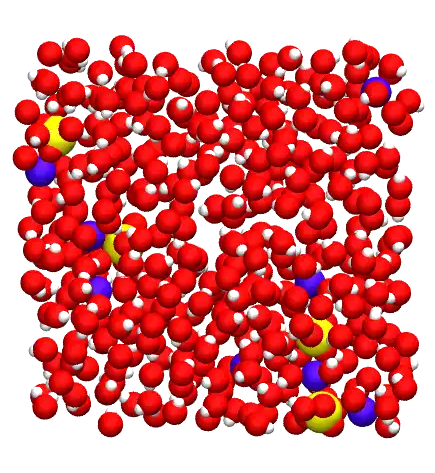
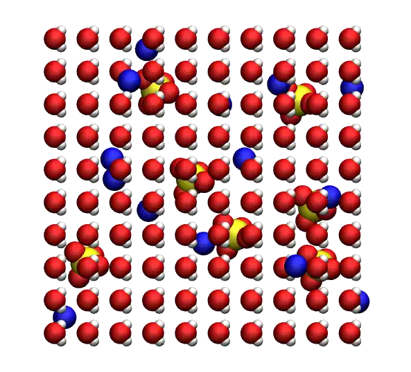
A conf.gro file can be visualized using VMD by typing in the terminal:
vmd conf.gro
This is what I see:
Figure: SO42- ions (in yellow and red) and Na+ ions (blue) in water (red and white).#
You have to play with atoms’ representation and color to make it look better than it is by default. I wrote a small VMD tutorial that explains how to obtain nice looking image.
As can be seen in this figure, the water molecules are arranged in a quite unrealistic and regular manner, with all dipoles facing in the same direction, and possibly wrong distances between some of the molecules and ions.
This will be fixed during energy minimization, see below.
2) The topology file (.top)#
If you already followed the previous tutorial, Write parameters, you can also skip this part.
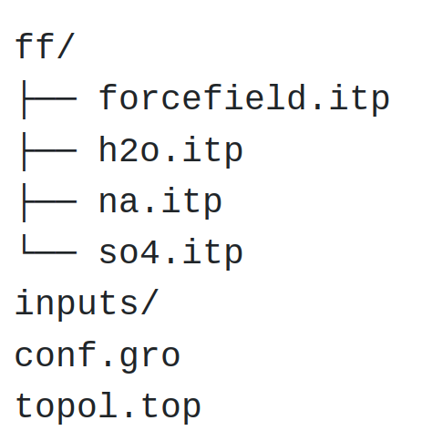
The topology file contains information about the interactions of the different atoms and molecules. You can download it by clicking here. Place it in the same folder as the conf.gro file. The topol.top file looks like that:
#include "ff/forcefield.itp"
#include "ff/h2o.itp"
#include "ff/na.itp"
#include "ff/so4.itp"

[ System ]
Na2SO4 solution

[ Molecules ]
SO4 6
Na 12
SOL 701
The 4 first lines are used to include the values of the parameters that are given in 4 separate files (see below).
The rest of the topol.top file contains the system name (Na2SO4 solution), and a list of the molecules. It is important that the order of the molecules in the topology file (here SO4 first, Na second, and SOL (H2O) last) matches the order of the conf.gro file, otherwise the simulation will fail.
Create a folder named ‘ff/’ next to the conf.gro and the topol.top files, and copy forcefield.itp, h2o.itp, na.itp, and so4.itp in it. These four files contain information about the atoms (names, masses, changes, Lennard-Jones coefficients) and residues (bond and angular constraints) for all the species that will be involved here.
3) The input file (.mdp)#
The input file contains instructions about the simulation, such as
the number of steps to perform,
the thermostat to be used (e.g. Langevin, Berendsen),
the cut-off for the interactions (e.g. Lennard-Jones),
the molecular dynamics integrator (e.g. steep-decent, molecular dynamics).
In this tutorial, 4 different input files will be written in order to perform respectively an energy minimization of the salt solution, an equilibration in the NVT ensemble (with fixed box sized), an equilibration in the NPT ensemble (with changing box size), and finally a production run. Input files will be placed in a ‘inputs/’ folder.
At this point, your folder should look like that:
The rest of the tutorial focusses on writing the input files and performing the molecular dynamics simulation.
Support me for 1 euro per month
Become a Patreon and support the creation of content for GROMACS
Energy minimization#
It is clear from the configuration (.gro) file that the molecules and ions are currently in a quite unphysical configuration (i.e. too regularly aligned). It would be risky to directly perform a molecular dynamics simulation; atoms would undergo huge forces, accelerate, and the system could eventually explode.
In order to bring the system into a favorable state, let us perform an energy minimization which consists in moving the atoms until the forces between them are reasonable.
Open a blank file, call it min.mdp, and save it in the ‘inputs/’ folder. Copy the following lines into min.mdp:
integrator = steep
nsteps = 5000
These commands specify to GROMACS that the algorithm to be used is the speepest-descent, which moves the atoms following the direction of the largest forces until one of the stopping criterial is reached. The ‘nsteps’ command specifies the maximum number of steps to perform.
In order to visualize the trajectory of the atoms during the minimization, let us add the following command to the input file in order to print the atom positions every 10 steps in a .trr trajectory file:
nstxout = 10
We now have a very minimalist input script, let us try it. From the terminal, type:
gmx grompp -f inputs/min.mdp -c conf.gro -p topol.top -o min -pp min -po min
gmx mdrun -v -deffnm min
The grompp command is used to preprocess the files in order to prepare the simulation. The grompp command also checks the validity of the files. By using the ‘-f’, ‘-c’, and ‘-p’ keywords, we specify which input, configuration, and topology files must be used, respectively. The other keywords ‘-o’, ‘-pp’, and ‘-po’ are used to specify the names of the output that will be produced during the run.
The mdrun command calls the engine performing the computation from the preprocessed files (which is recognized thanks to the -deffnm keyword). The ‘-v’ option is here to enable verbose and have more information printed in the terminal.
If everything works, you should see something like :
(...)

Steepest Descents converged to machine precision in 824 steps,
but did not reach the requested Fmax < 10.
Potential Energy  = -6.8990930e+04
Maximum force     =  2.4094606e+02 on atom 1654
Norm of force     =  4.6640654e+01
The information printed in the terminal indicates us that energy minimization has been performed, even though the precision that was asked from the default parameters was not reached. We can ignore this message, as long as the final energy is large and negative, the simulation will work just fine.
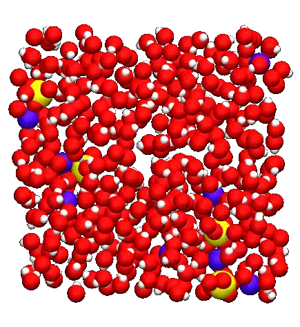
The final potential energy is large and negative, and the maximum force is small: 240 kJ/mol/nm (about 0.4 pN). Everything seems alright. Let us visualize the atoms’ trajectories during the minimization step using VMD by typing in the terminal:
vmd conf.gro min.trr
This is what I see:
Note for VMD user: You can avoid having molecules ‘cut in half’ by the periodic boundary conditions by rewriting the trajectory using ‘gmx trjconv -f min.trr -s min.tpr -o min_whole.trr -pbc whole’
One can see that the molecules reorient themselves into more energetically favorable positions, and that the distances between the atoms are being progressively homogeneized.
Let us have a look at the evolution of the potential energy of the system. To do so, we can use the internal ‘energy’ command of GROMACS. In the terminal, type:
gmx energy -f min.edr -o epotmin.xvg
choose ‘potential’ by typing ‘5’ (or any number that is in front of ‘potential’), then press enter twice.
Here the edr file produced by Gromacs during the last run is used, and the result is saved in the epotmin.xvg file. Let us plot it (xvg files can be easily opened using XmGrace, here I use pyplot and jupyter-notebook):
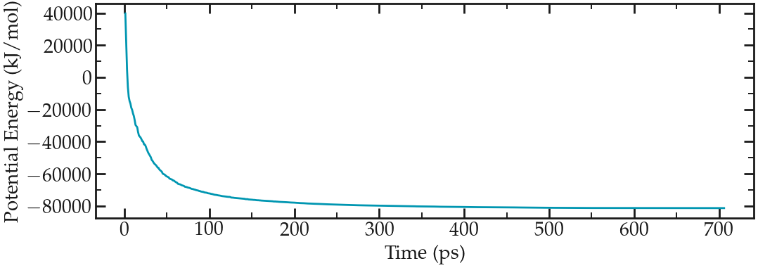
Evolution of the potential energy as a function of the number of steps during energy minimization.#
One can see from the energy plot that the potential energy is initially huge and positive, which is the consequence of atoms being too close from one another, as well as molecules being wrongly oriented. As the minimization progresses, the potential energy rapidly decreases and reaches a large and negative value, which is usually a good sign as it indicates that the atoms are now at appropriate distances from each others.
The system is ready for the molecular dynamics simulation.
Minimalist NVT input file#
Let us first perform a small (20 picoseconds) equilibration in the NVT ensemble. In the NVT ensemble, the number of atom (N) and volume (V) are maintained fixed, and the temperature (T) is adjusted using a thermostat.
Let use write a new input script called nvt.mdp, and save it in the ‘inputs/’ folder. Copy the following lines into it:
integrator = md
nsteps = 20000
dt = 0.001
Here the molecular dynamics (md) integrator is used (leapfrog algorithm), and a number of 20000 steps with timestep (dt) 0.001 ps is requested, so the total requested duration is 20 ps. Let us print the trajectory in a xtc file every 1 ps by adding:
nstxout-compressed = 1000
Let us control the temperature over the course of the simulation using the v-rescale thermostat, which is the Berendsen thermostat with an additional stochastic term (it is known to give proper canonical ensemble):
tcoupl = v-rescale
ref-t = 360
tc-grps = system
tau-t = 0.5
Here we also specified that the thermostat is applied to the entire system (we could choose to apply it only to a certain group of atom, which we will do later), and that the damping constant for the thermostat is 0.5 ps.
Note that the relatively high temperature of 360 K has been chosen here in order to reduce the viscosity of the solution and converge toward the desired result (i.e. the diffusion coefficient) faster. We now have a minimalist input file for performing the NVT step. Run it by typing in the terminal:
gmx grompp -f inputs/nvt.mdp -c min.gro -p topol.top -o nvt -pp nvt -po nvt
gmx mdrun -v -deffnm nvt
Here ‘-c min.gro’ ensures that the previously minimized configuration is used as a starting point.
After the completion of the simulation, we can ensure that the system temperature indeed reached the value of 360 K by using the energy command of GROMACS. Type:
gmx energy -f nvt.edr -o Tnvt.xvg
and choose ‘temperature’.
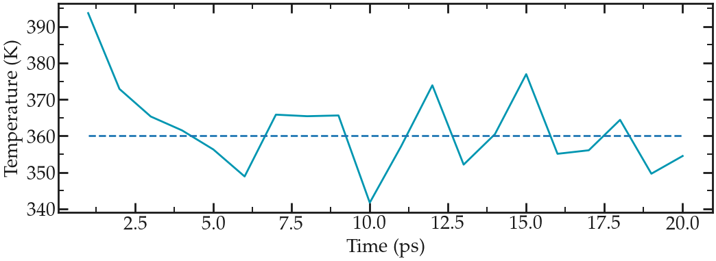
From the generated file, we can see that temperature started from 0, which was expected since the atoms have no velocity during a minimization step, and reaches a temperature slightly larger than the requested 360 K after a duration of a few picoseconds:
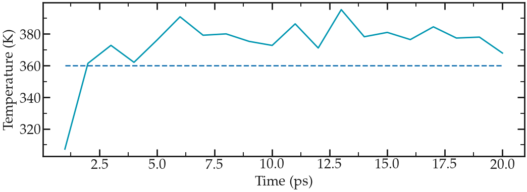
Evolution of the temperature as a function of the time during the NVT equilibration. Dashed line is the requested temperature of 360 K.#
A better control of the temperature is achieved in the next section.
Improving the NVT#
So far, a very few commands have been placed in the NVT input file, meaning that most of the instruction have been taken by GROMACS from the default parameters. You can find what parameters were used during the last nvt run by opening the new nvt.mdp file that has been created (i.e. not the one in the ‘inputs/’ folder, but the one in the main folder). Exploring this new nvt.mdp file shows us that, for instance, plain cut-off Coulomb interactions have been used:
; Method for doing electrostatics
coulombtype = Cut-off
For this system, long range Coulomb interaction is a better choice. We could also improve the thermostating of the system by applying a separate thermostat to water molecules and ions. Therefore, let us improve the NVT step by specifying more options in the input file. First, in the nvt.mdp file, let us impose the use of the long-range Fast smooth Particle-Mesh Ewald (SPME) electrostatics with Fourier spacing of 0.1 nm, order of 4, and cut-off of 4:
coulombtype = pme
fourierspacing = 0.1
pme-order = 4
rcoulomb = 1.0
Note that with PME, the cut-off specifies which interactions are treated with Fourier transforms. Let us also specify the van der Waals interaction:
vdw-type = Cut-off
rvdw = 1.0
as well as the constraint algorithm for the hydrogen bonds of the water molecules:
constraint-algorithm = lincs
constraints = hbonds
continuation = no
Let us also use separate temperature baths for water and ions (here corresponding to the gromacs group called non-water) respectively by replacing:
tcoupl = v-rescale
ref-t = 360
tc-grps = system
tau-t = 0.5
by:
tcoupl = v-rescale
tc-grps = Water non-Water
tau-t = 0.5 0.5
ref-t = 360 360
Let us specify neighbor searching parameters:
cutoff-scheme = Verlet
nstlist = 10
ns_type = grid
Let us give an initial kick to the atom (so that the initial total velocities give the desired temperature instead of 0):
gen-vel = yes
gen-temp = 360
and let us remove center of mass translational velocity of the whose system:
comm_mode = linear
comm_grps = system
Run the new version of the input script. One obvious difference with the previous (minimalist) NVT run is the temperature at the beginning of the run (orange curve). The final temperature is also closer to the desired temperature:
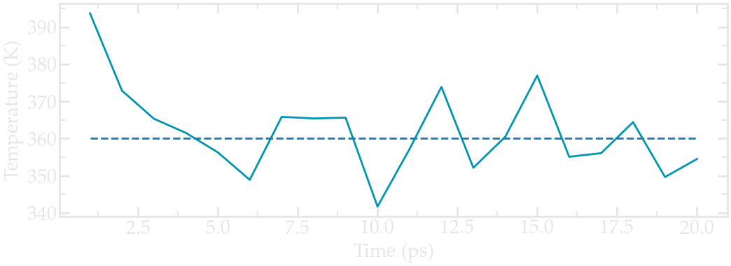
Evolution of the temperature as a function of the time during the NVT equilibration.#
Adjust the density using NPT#
Now that the system is properly equilibrated in the NVT ensemble, let us perform an equilibration in the NPT ensemble, where the pressure is imposed and the volume of the box is free to relax. NPT relaxation ensures that the density of the fluid converges toward its equilibrium value. Create a new input script, call it ‘npt.mdp’, and copy the following lines in it:
integrator = md
nsteps = 50000
dt = 0.001

comm_mode = linear
comm_grps = system

cutoff-scheme = Verlet
nstlist = 10
ns_type = grid

nstlog = 100
nstenergy = 100
nstxout-compressed = 1000

vdw-type = Cut-off
rvdw = 1.0

coulombtype = pme
fourierspacing = 0.1
pme-order = 4
rcoulomb = 1.0

constraint-algorithm = lincs
constraints = hbonds

tcoupl = v-rescale
ld-seed = 48456
tc-grps = Water non-Water
tau-t = 0.5 0.5
ref-t = 360 360

pcoupl = C-rescale
Pcoupltype = isotropic
tau_p = 1.0
ref_p = 1.0
compressibility = 4.5e-5
The main difference with the previous NVT script, is the addition of the isotropic C-rescale pressure coupling with a target pressure of 1 bar. Some other differences are the addition of the ‘nstlog’ and ‘nstenergy’ commands to control the frequency at which information are printed in the log file and in the energy file (edr), and the removing the ‘gen-vel’ commands. Run it using:
gmx grompp -f inputs/npt.mdp -c nvt.gro -p topol.top -o npt -pp npt -po npt
gmx mdrun -v -deffnm npt
Let us have a look a both temperature, pressure and volume during the NPT step using the ‘gmx energy’ command 3 times:
gmx energy -f npt.edr -o Tnpt.xvg
gmx energy -f npt.edr -o Pnpt.xvg
gmx energy -f npt.edr -o Vnpt.xvg
Choose respectively ‘temperature’, ‘pressure’ and ‘volume’. This is what I see:
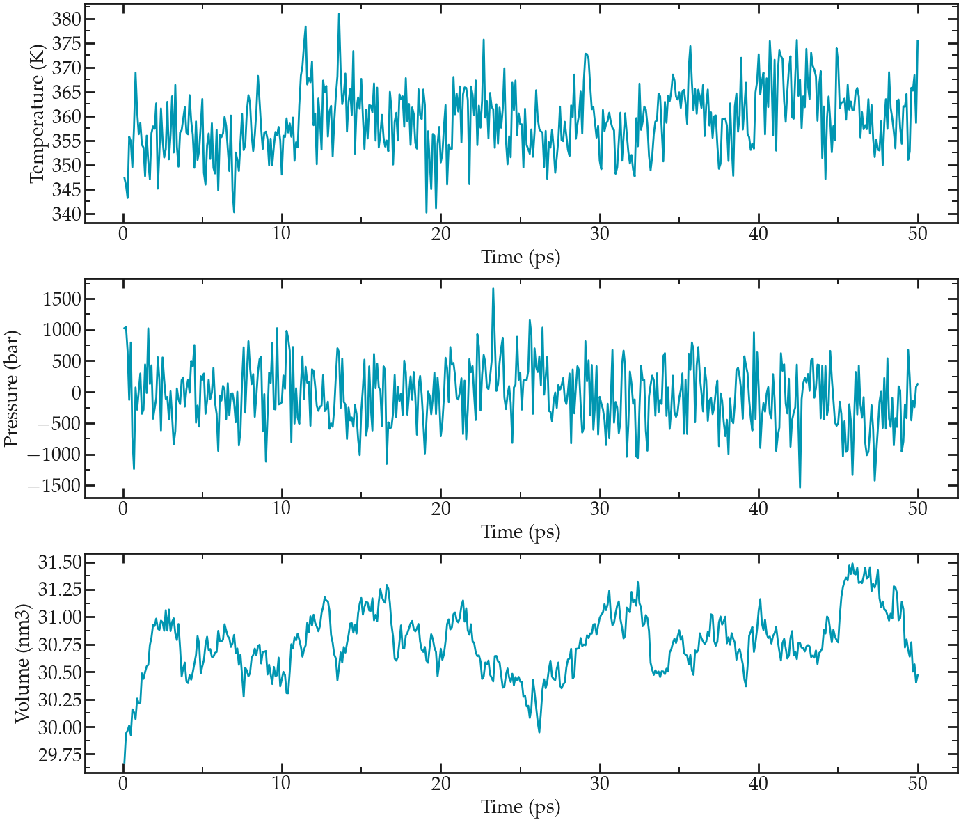
From top to bottom: evolution of the temperature, pressure, and volume of the simulation box as a function of the time during the NPT equilibration.#
The results show that the temperature remains well controlled during the NPT run. The results also show that the volume was initially too small for the desired pressure, and equilibrated itself at a slightly larger value after a few pico-seconds. Finally, the pressure curve reveal that large oscillations of the pressure with time. These large oscillations are typical in molecular dynamics, particularly with liquid water that is almost uncompressible.
Exact results may differ depending on the actual .gro file generated.
Measurement diffusion coefficient#
Now that the system is fully equilibrated, we can perform a longer simulation and extract quantities of interest.
Here, as an illustration, the diffusion coefficients of all 3 species (water and the two ions) will be measured. First, let us perform a longer run in the NVT ensemble. Create a new input file, call it ‘pro.mdp’ (‘pro’ is short for ‘production’), and copy the following lines into it:
integrator = md
nsteps = 200000
dt = 0.001

comm_mode = linear
comm_grps = system

cutoff-scheme = Verlet
nstlist = 10
ns_type = grid

nstlog = 100
nstenergy = 100
nstxout-compressed = 1000

vdw-type = Cut-off
rvdw = 1.0

coulombtype = pme
fourierspacing = 0.1
pme-order = 4
rcoulomb = 1.0

constraint-algorithm = lincs
constraints = hbonds

tcoupl = v-rescale
ld-seed = 48456
tc-grps = Water non-Water
tau-t = 0.5 0.5
ref_t = 360 360
Run it using:
gmx grompp -f inputs/pro.mdp -c npt.gro -p topol.top -o pro -pp pro -po pro
gmx mdrun -v -deffnm pro
When its completed, compute the mean square displacement using:
gmx msd -f pro.xtc -s pro.tpr -o SO4.xvg
and select the SO4 ions by typing ‘SO4’, and then press ‘ctrl D’.
Fitting the slope of the MSD gives a value of 1.3e-5 cm2/s for the diffusion coefficient.
Repeat the same for Na and water.
For Na, the value is 1.5e-5 cm2/s, and for water 5.2e-5 cm2/s (not too far from the experimental value of ~ 7e-5 cm2/s at temperature T=360 K).
About MSD in molecular simulations
In principle, diffusion coefficients obtained from molecular dynamics simulations in a finite-sized box must be corrected, but this is beyond the scope of the present tutorial, see this paper for more details.
The final MSDs plots look like this:
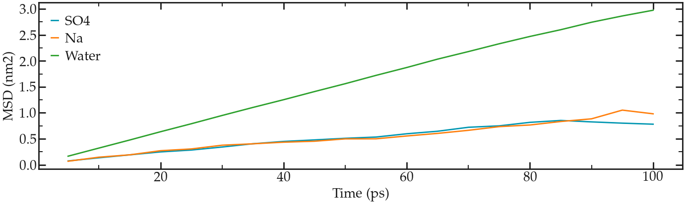
MSDs for the three species, respectively.#
Going further#
Take advantage of the generated production run to extract more equilibrium quantities. For instance, Gromacs allows you to extract Radial Distribution Functions (RDF) using the gmx rdf commands.
Contact me
Contact me if you have any question or suggestion about these tutorials.